Analysis of Variance (ANOVA) and Analysis of Covariance (ANCOVA)
Analysis of variance (ANOVA) is a collection of statistical models and their associated estimation procedures (such as the "variation" among and between groups) used to analyze the differences among group means in a sample. ANOVA was developed by statistician and evolutionary biologist Ronald Fisher. In the ANOVA setting, the observed variance in a particular variable is partitioned into components attributable to different sources of variation. In its simplest form, ANOVA provides a statistical test of whether the population means of several groups are equal, and therefore generalizes the t-test to more than two groups. ANOVA is useful for comparing (testing) three or more group means for statistical significance. It is conceptually similar to multiple two-sample t-tests, but is more conservative, resulting in fewer type I errors,[1] and is therefore suited to a wide range of practical problems.
In the typical application of ANOVA, the null hypothesis is that all groups are random samples from the same population. For example, when studying the effect of different treatments on similar samples of patients, the null hypothesis would be that all treatments have the same effect (perhaps none). Rejecting the null hypothesis is taken to mean that the differences in observed effects between treatment groups are unlikely to be due to random chance.
One-way analysis of covariance (ANCOVA) is similar to ANOVA in that two or more groups are being compared on the mean of some dependent variable, but ANCOVA additionally controls for a variable (covariate) that may influence the DV (e.g., Do preschoolers of low, middle, and high socioeconomic status [IV] have different literacy test scores [DV] after adjusting for family type [covariate]?). Many times the covariate may be pretreatment differences in which groups are equated in terms of the covariate(s). In general, ANCOVA is appropriate when the IV is defined as having two or more categories, the DV is quantitative, and the effects of one or more covariates need to be removed.
ANOVA Example: Weight versus age of chicks on different diets
Description: The body weights of the chicks were measured at birth and every second day thereafter until day 20. They were also measured on day 21. There were four groups on chicks on different protein diets.
weight: body weight of the chick in grams.
time: number of days since birth when the measurement was made.
chick: a numerical identifier of each chick
diet: a factor with levels 1, ..., 4 indicating which experimental diet the chick received.
Source: https://vincentarelbundock.github.io/Rdatasets/doc/datasets/ChickWeight.html
Download the data from here
Task: Is there a difference among diets?
Here we will test whether weight distribution changes with different diets. Therefore our classification variable is diet and test variable is weight. We can put this information into PROC FORMAT like this:
								PROC ANOVA DATA = tutorial.chickweight;

								CLASS diet;

								MODEL weight = diet;

								RUN;
| Source | DF | Sum of Squares | Mean Square | F Value | Pr > F |
|---|---|---|---|---|---|
| Model | 3 | 155862.658 | 51954.219 | 10.81 | <.0001 |
| Error | 574 | 2758693.268 | 4806.086 | ||
| Corrected Total | 577 | 2914555.926 |
| R-Square | Coeff Var | Root MSE | weight Mean |
|---|---|---|---|
| 0.053477 | 56.90928 | 69.32594 | 121.8183 |
| Source | DF | Anova SS | Mean Square | F Value | Pr > F |
|---|---|---|---|---|---|
| Diet | 3 | 155862.6576 | 51954.2192 | 10.81 | <.0001 |
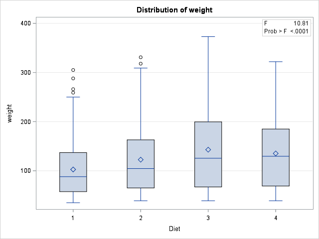
p-value for F-test tells us that at least one of the diets is different. But what about individual differences? We can find these with SCHEFFE test (other option is TUKEY):
								PROC ANOVA DATA = tutorial.chickweight;

								CLASS diet;

								MODEL weight = diet / TUKEY;

								RUN;
| Note: | This test controls the Type I experimentwise error rate, but it generally has a higher Type II error rate than Tukey's for all pairwise comparisons. |
| Alpha | 0.05 |
|---|---|
| Error Degrees of Freedom | 574 |
| Error Mean Square | 4806.086 |
| Critical Value of F | 2.62043 |
| Comparisons significant at the 0.05 level are indicated by ***. |
||||
|---|---|---|---|---|
| Diet Comparison |
Difference Between Means |
Simultaneous 95% Confidence Limits |
||
| 3 - 4 | 7.687 | -17.513 | 32.887 | |
| 3 - 2 | 20.333 | -4.760 | 45.427 | |
| 3 - 1 | 40.305 | 18.246 | 62.363 | *** |
| 4 - 3 | -7.687 | -32.887 | 17.513 | |
| 4 - 2 | 12.646 | -12.554 | 37.846 | |
| 4 - 1 | 32.617 | 10.438 | 54.797 | *** |
| 2 - 3 | -20.333 | -45.427 | 4.760 | |
| 2 - 4 | -12.646 | -37.846 | 12.554 | |
| 2 - 1 | 19.971 | -2.087 | 42.030 | |
| 1 - 3 | -40.305 | -62.363 | -18.246 | *** |
| 1 - 4 | -32.617 | -54.797 | -10.438 | *** |
| 1 - 2 | -19.971 | -42.030 | 2.087 | |
SCHEFFE test tells us that Diet 1 and Diets 3-4 are significantly different. Diets 2, 3 and 4 are not statistically different.
ANCOVA Example (1 CoVar): Potency of two herbicides
Description: Data are from an experiment, comparing the potency of the two herbicides glyphosate and bentazone in white mustard Sinapis alba.
dose: a numeric vector containing the dose in g/ha.
herbicide: a factor with levels Bentazone Glyphosate (the two herbicides applied).
drymatter: a numeric vector containing the response (dry matter in g/pot).
Source: https://vincentarelbundock.github.io/Rdatasets/doc/drc/S.alba.html
Download the data from here
Task: Are there any significant differences between herbicides?
If we hadn't have a column called 'dose', this would have been an ANOVA case however effect of dose cannot be ignored therefore we need to apply ANCOVA instead. We can do an ANCOVA analysis via PROC GLM:
								PROC GLM DATA = tutorial.salba;

								CLASS herbicide;

								MODEL drymatter = dose herbicide / SOLUTION;

								LSMEANS herbicide / STDERR PDIFF COV;

								RUN;
| Class Level Information | ||
|---|---|---|
| Class | Levels | Values |
| Herbicide | 2 | Bentazone Glyphosate |
| Number of Observations Read | 68 |
|---|---|
| Number of Observations Used | 68 |
| Source | DF | Sum of Squares | Mean Square | F Value | Pr > F |
|---|---|---|---|---|---|
| Model | 2 | 67.7937369 | 33.8968684 | 30.20 | <.0001 |
| Error | 65 | 72.9537631 | 1.1223656 | ||
| Corrected Total | 67 | 140.7475000 |
| R-Square | Coeff Var | Root MSE | DryMatter Mean |
|---|---|---|---|
| 0.481669 | 43.68732 | 1.059418 | 2.425000 |
| Source | DF | Type I SS | Mean Square | F Value | Pr > F |
|---|---|---|---|---|---|
| Dose | 1 | 65.62087826 | 65.62087826 | 58.47 | <.0001 |
| Herbicide | 1 | 2.17285862 | 2.17285862 | 1.94 | 0.1689 |
| Source | DF | Type III SS | Mean Square | F Value | Pr > F |
|---|---|---|---|---|---|
| Dose | 1 | 59.00804244 | 59.00804244 | 52.57 | <.0001 |
| Herbicide | 1 | 2.17285862 | 2.17285862 | 1.94 | 0.1689 |
| Parameter | Estimate | Standard Error |
t Value | Pr > |t| | |
|---|---|---|---|---|---|
| Intercept | 3.255259183 | B | 0.19725274 | 16.50 | <.0001 |
| Dose | -0.005701704 | 0.00078635 | -7.25 | <.0001 | |
| Herbicide Bentazone | -0.364574298 | B | 0.26202184 | -1.39 | 0.1689 |
| Herbicide Glyphosate | 0.000000000 | B | . | . | . |
| Herbicide | DryMatter LSMEAN | Standard Error |
H0:LSMEAN=0 | H0:LSMean1=LSMean2 |
|---|---|---|---|---|
| Pr > |t| | Pr > |t| | |||
| Bentazone | 2.25343562 | 0.17807119 | <.0001 | 0.1689 |
| Glyphosate | 2.61800992 | 0.18907116 | <.0001 |
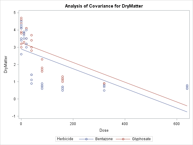
We can see from the results that while there is some difference between herbicides, it's not enough to achieve statistical significance as evident from p-value (0.1689). Also note that we used LSMEANS instead of MEANS as this is preferable in ANCOVA models.
ANCOVA Example (2 CoVars): Epiliptic Seizures
Description: The seizure data frame has 59 rows and 7 columns. The dataset has the number of epiliptic seizures in a new eight-week interval, and in a baseline eight-week inverval, for treatment and control groups with a total of 59 individuals.
trt: An indicator of treatment.
age: Age in years.
pre: The number of epilitic seizures in a baseline 8-week interval.
post: The number of epilitic seizures in a new 8-week interval.
Source: https://vincentarelbundock.github.io/Rdatasets/doc/geepack/seizure.html
Download the data from here
Task: Is the treatment effective?
								PROC GLM DATA = tutorial.seizure;

								CLASS trt;

								MODEL post = pre age trt / SOLUTION;

								LSMEANS trt / STDERR PDIFF COV;

								RUN;
| Source | DF | Sum of Squares | Mean Square | F Value | Pr > F |
|---|---|---|---|---|---|
| Model | 3 | 84474.3036 | 28158.1012 | 43.03 | <.0001 |
| Error | 55 | 35988.2727 | 654.3322 | ||
| Corrected Total | 58 | 120462.5763 |
| R-Square | Coeff Var | Root MSE | post Mean |
|---|---|---|---|
| 0.701249 | 77.31635 | 25.57992 | 33.08475 |
| Source | DF | Type I SS | Mean Square | F Value | Pr > F |
|---|---|---|---|---|---|
| pre | 1 | 83201.74674 | 83201.74674 | 127.16 | <.0001 |
| age | 1 | 1078.99227 | 1078.99227 | 1.65 | 0.2045 |
| trt | 1 | 193.56456 | 193.56456 | 0.30 | 0.5887 |
| Source | DF | Type III SS | Mean Square | F Value | Pr > F |
|---|---|---|---|---|---|
| pre | 1 | 84016.56359 | 84016.56359 | 128.40 | <.0001 |
| age | 1 | 1063.57862 | 1063.57862 | 1.63 | 0.2077 |
| trt | 1 | 193.56456 | 193.56456 | 0.30 | 0.5887 |
| Parameter | Estimate | Standard Error |
t Value | Pr > |t| | |
|---|---|---|---|---|---|
| Intercept | -30.05147408 | B | 14.86419774 | -2.02 | 0.0481 |
| pre | 1.43864132 | 0.12696068 | 11.33 | <.0001 | |
| age | 0.57111075 | 0.44795531 | 1.27 | 0.2077 | |
| trt 0 | 3.62823331 | B | 6.67085405 | 0.54 | 0.5887 |
| trt 1 | 0.00000000 | B | . | . | . |
| trt | post LSMEAN | H0:LSMean1=LSMean2 |
|---|---|---|
| Pr > |t| | ||
| 0 | 34.9911056 | 0.5887 |
| 1 | 31.3628723 |
As seen from the results above (p=0.5887 > 0.05), the treatment is not effective.

Lrrr
Senior blog writer
Lrrr, ruler of the planet Omicron Persei 8, is a middle-aged Omicronian man with a bad temper and soft spots for the conquering of planets and 20th century television.
Popular Posts

Space The Final Frontier
02 Hours ago

The Amazing Hubble
02 Hours ago

Astronomy Or Astrology
02 Hours ago

Asteroids telescope
02 Hours ago

Leave a Comment