Logistic Regression with SAS PROC LOGISTIC

Logistic Regression

Logistic model (or logit model) is a widely used statistical model that, in its basic form, uses a logistic function to model a binary dependent variable; many more complex extensions exist. In regression analysis, logistic regression (or logit regression) is estimating the parameters of a logistic model; it is a form of binomial regression. Mathematically, a binary logistic model has a dependent variable with two possible values, such as pass/fail, win/lose, alive/dead or healthy/sick; these are represented by an indicator variable, where the two values are labeled "0" and "1".

Logistic regression is used in various fields, including machine learning, most medical fields, and social sciences. For example, the Trauma and Injury Severity Score (TRISS), which is widely used to predict mortality in injured patients, was originally developed by Boyd et al. using logistic regression. Many other medical scales used to assess severity of a patient have been developed using logistic regression.Logistic regression may be used to predict the risk of developing a given disease (e.g. diabetes; coronary heart disease), based on observed characteristics of the patient (age, sex, body mass index, results of various blood tests, etc.). It is also used in marketing applications such as prediction of a customer's propensity to purchase a product or halt a subscription, etc. In economics it can be used to predict the likelihood of a person's choosing to be in the labor force, and a business application would be to predict the likelihood of a homeowner defaulting on a mortgage. Conditional random fields, an extension of logistic regression to sequential data, are used in natural language processing.

Example: Frogs

Description: This data frame gives the distribution of the Southern Corroboree frog, which occurs in the Snowy Mountains area of New South Wales, Australia.

pres.abs: 0 = frogs were absent, 1 = frogs were present
northing: reference point.
easting: reference point.
altitude: altitude in meters.
distance: distance in meters to nearest extant population.
noofpools: number of potential breeding pools.
noofsites: number of potential breeding sites within a 2 km radius.
avrain: mean rainfall for Spring period.
meanmin: mean minimum Spring temperature.
meanmax: mean maximum Spring temperature.

Source: https://vincentarelbundock.github.io/Rdatasets/doc/DAAG/frogs.html
Download the data from here

Task: What are the best parameters for existence of frogs?

Let's begin our first shot at our logistic model. At first, we will include all the possible independent variables:

Model I

							
								PROC LOGISTIC DATA = tutorial.frogs;

								CLASS pres_abs;

								MODEL pres_abs = northing easting altitude distance noofpools noofsites avrain meanmin meanmax;

								RUN;

The LOGISTIC Procedure

Model Information
Data Set	TUTORIAL.FROGS
Response Variable	pres_abs
Number of Response Levels	2
Model	binary logit
Optimization Technique	Fisher's scoring

Number of Observations Read	212
Number of Observations Used	212

Response Profile
Ordered Value	pres_abs	Total Frequency
1	0	133
2	1	79

Probability modeled is pres_abs='0'.

Model Convergence Status
Convergence criterion (GCONV=1E-8) satisfied.

Model Fit Statistics
Criterion	Intercept Only	Intercept and Covariates
AIC	281.987	215.660
SC	285.344	249.226
-2 Log L	279.987	195.660

Testing Global Null Hypothesis: BETA=0
Test	Chi-Square	DF	Pr > ChiSq
Likelihood Ratio	84.3270	9	<.0001
Score	65.7949	9	<.0001
Wald	42.4876	9	<.0001

Analysis of Maximum Likelihood Estimates
Parameter	DF	Estimate	Standard Error	Wald Chi-Square	Pr > ChiSq
Intercept	1	163.5	215.3	0.5765	0.4477
northing	1	-0.0104	0.0165	0.3964	0.5290
easting	1	0.0216	0.0127	2.8974	0.0887
altitude	1	-0.0709	0.0770	0.8466	0.3575
distance	1	0.000483	0.000206	5.5057	0.0190
NoOfPools	1	-0.0297	0.00944	9.8782	0.0017
NoOfSites	1	-0.0430	0.1095	0.1541	0.6946
avrain	1	0.000039	0.1300	0.0000	0.9998
meanmin	1	-15.6444	6.4785	5.8313	0.0157
meanmax	1	-1.7066	6.8087	0.0628	0.8021

Under "Testing Global Null Hypothesis: BETA=0" section, we see that p-values are all significant. In practice, this really doesn't mean much - it just proves that our model is better than intercept only. I I call this measure as "better than nothing" test. Now let's look into individual variables under 'Analysis of Maximum Likelihood Estimates'.

Based on our p-values, distance, noofpools and meanmin are the relevant parameters. So we shall drop the other parameters and we're done, right? Unfortunately not. What this results tells us that distance, noofpools and meanmin are the most important variables within the set of variables in our model. That is, if this combination of variables (variables specified after MODEL statement) are the best there is then yes, we're done. But what about interaction terms? We haven't included them in our model. To include them in our model, we can specify them as var1 var2 var1*var2 or simply var1|var2. Let's include northing|easting and meanmin|meanmax. Before that note our SC measure under Model Fit Statistics; the lower this number the better. SC for our first model 249.226. We can compare this number with the SC values all the models we will develop. We could also use AIC or -2Log L. SC tends to penalize a high number of independent variables more than AIC and less than -2Log L, therefore we will use SC for this study.

Model II

							
								PROC LOGISTIC DATA= tutorial.frogs;

								CLASS pres_abs;

								MODEL pres_abs = northing|easting altitude distance noofpools noofsites avrain meanmin|meanmax;

								RUN;

Let's look at our results:

Model Fit Statistics
Criterion	Intercept Only	Intercept and Covariates
AIC	281.987	217.295
SC	285.344	257.574
-2 Log L	279.987	193.295

Analysis of Maximum Likelihood Estimates
Parameter	DF	Estimate	Standard Error	Wald Chi-Square	Pr > ChiSq
Intercept	1	305.9	245.3	1.5543	0.2125
northing	1	-0.1774	0.1360	1.7028	0.1919
easting	1	-0.0251	0.0354	0.5023	0.4785
northing*easting	1	0.000148	0.000116	1.6119	0.2042
altitude	1	-0.0592	0.0784	0.5706	0.4500
distance	1	0.000417	0.000210	3.9539	0.0468
NoOfPools	1	-0.0307	0.00999	9.4480	0.0021
NoOfSites	1	-0.0732	0.1141	0.4109	0.5215
avrain	1	-0.2638	0.2410	1.1980	0.2737
meanmin	1	-19.0926	6.9116	7.6308	0.0057
meanmax	1	-8.2044	8.0896	1.0286	0.3105
meanmin*meanmax	1	0.6919	0.4816	2.0643	0.1508

Allright, so far our results are similar to the previous one - distance, noofpools and meanmin are the relevant parameters, again. Our SC is 257.574 higher than our previous model. Therefore we can discard our current model and go back to the first model and remove unrelevant variables. And one more thing: SAS by default calculates odd ratios for dependent = 0, i.e. pres_abs = 0. To change this we need to specify the event as 1 like the following.

Model III

							
								PROC LOGISTIC DATA= tutorial.frogs;

								CLASS pres_abs;

								MODEL pres_abs(EVENT = '1') = distance noofpools meanmin;

								RUN;

Model Fit Statistics
Criterion	Intercept Only	Intercept and Covariates
AIC	281.987	224.104
SC	285.344	237.530
-2 Log L	279.987	216.104

Analysis of Maximum Likelihood Estimates
Parameter	DF	Estimate	Standard Error	Wald Chi-Square	Pr > ChiSq
Intercept	1	-4.6333	1.1465	16.3318	<.0001
distance	1	-0.00060	0.000173	12.0480	0.0005
NoOfPools	1	0.0251	0.00807	9.6855	0.0019
meanmin	1	1.3438	0.3087	18.9499	<.0001

Odds Ratio Estimates
Effect	Point Estimate	95% Wald Confidence Limits
distance	0.999	0.999	1.000
NoOfPools	1.025	1.009	1.042
meanmin	3.834	2.093	7.021

Association of Predicted Probabilities and Observed Responses
Percent Concordant	81.9	Somers' D	0.638
Percent Discordant	18.1	Gamma	0.638
Percent Tied	0.0	Tau-a	0.300
Pairs	10507	c	0.819

Our SC is 237.530, lowest of all models. Note that if you are looking for a R-Square value, there is none in logistic regression but Tau-a value can be taken as a similar value. We are looking for high Tau-a values in logistic regression, similar to R-Sq in ordinary linear regressions. Now let's take a look at our odds ratio estimates.

For distance, every 1 unit increase in distance results in (0.999-1=-0.001) 0.1% decreased chance of finding frogs. Similarly, every additional noofpools results in (1.025-1=0.025) 2.5% increased chance and every additional meanmin results in (3.834-1=2.834) 283% increased chance of finding frogs. Let's graphically verify these with PROC KDE:

							
								PROC KDE DATA= tutorial.frogs;

								BIVAR distance noofpools /PLOTS = CONTOUR;

								FREQ pres_abs;

								RUN;

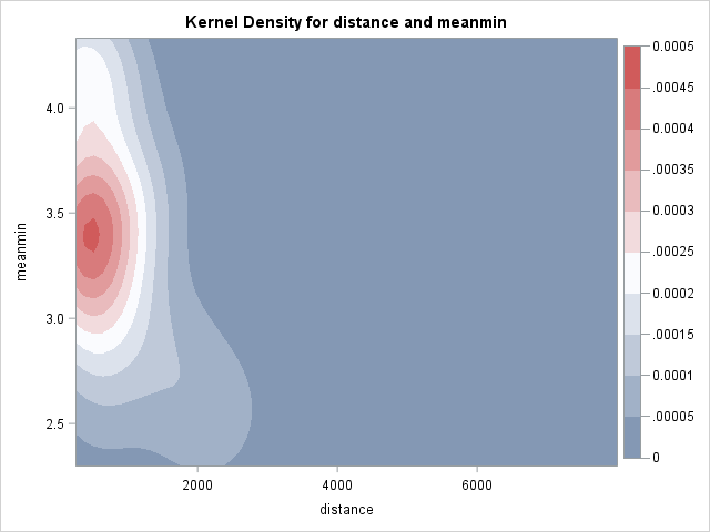
Here is our first problem. It seems like there is a decrease in frog population with increased distance, as expected, whereas the same cannot be said about meanmin. It looks like there is an optimum point around 3.5 and frog population decrease above and below this point. This is a sign of non-linearity. Also we can see that distance effect might not be linear either. We can see the whether there is any non-linear effect with EFFECTPLOT FIT statement:

							
								PROC LOGISTIC DATA=tutorial.frogs;

								CLASS pres_abs;

								MODEL pres_abs = distance noofpools meanmin;

								EFFECTPLOT FIT(X=distance);

								RUN;

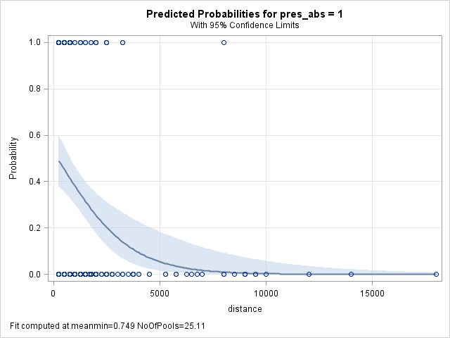
It can be seen from above that the effect is hardly linear. Let's make a logarithmic transormation of distance and try it again:

Model IV

							
								DATA tutorial.frogs;

								SET tutorial.frogs;

								logdistance = LOG(sitance);

								PROC LOGISTIC DATA = tutorial.frogs;

								CLASS pres_abs;

								MODEL pres_abs = logdistance noofpools meanmin;

								EFFECTPLOT FIT(X=logdistance);

								RUN;

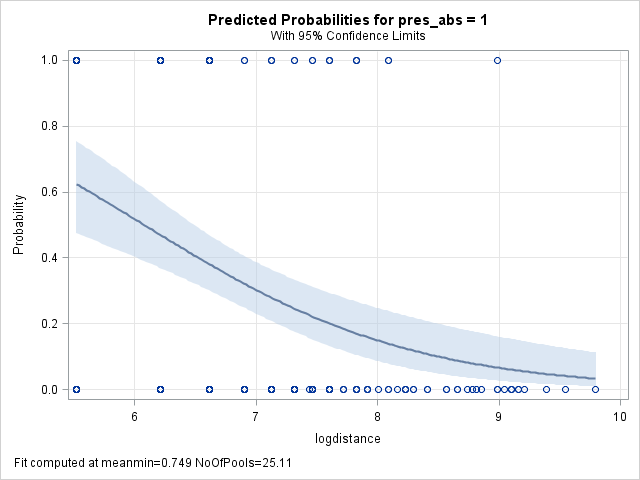
OK, looks like we are on the right track. And what about meanmin? It is clear from our PROC KDE graph that meanmin has an optimum point, therefore we can transform this variable to optimum point - meanmin. Finding the optimum point, however, is a little bit complicated. For this we need to run logistic regression with x - meanmin for various x's and pick the one which yields the lowest SC. SAS lets us do this with macros. Here is the macro I used for this purpose:

							
								%MACRO findopt(begin,n,interval);

								%DO i=1 %TO &n;

								     DATA frogs;

								     SET tutorial.frogs;

								     meanminopt = ABS(&begin + &i * &interval - meanmin);

								     CALL SYMPUT("x", &begin + &interval * &i);

								     PROC LOGISTIC DATA=frogs;

								     CLASS pres_abs;

								     MODEL pres_abs(EVENT="1") = logdistance meanminopt noofpools;

								     ODS OUTPUT FitStatistics = Fit&i;

								     RUN;

								     DATA fit&i;

								     SET fit&i;

								     IF criterion NE "SC" THEN DELETE;

								     x = &x;

								     DROP InterceptOnly;

								     DATA fit;

								     SET fit fit&i;

								%END;

								PROC SORT DATA = fit OUT = fitsort NODUPRECS;

								BY InterceptAndCovariates;

								RUN;

								DATA fitsort;

								SET fitsort;

								IF _n_ < 2 THEN CALL SYMPUT("optpoint",x);

								DATA frogs;

								SET frogs;

								meanminopt = ABS(&optpoint - meanmin);

								PROC LOGISTIC DATA = frogs;

								CLASS pres_abs;

								MODEL pres_abs(EVENT="1") = logdistance meanminopt noofpools;

								%MEND;

To run the macro, we simply call it with a percentage sign:

							
								%findopt(3.1,60,0.02);

We found that optimum point is 3.72. To verify this graphically:

							
								PROC SGPLOT DATA = fit;

								SERIES X=x Y=InterceptAndCovariates / MARKERS;

								RUN;

Here's our final model output:

Model V

The LOGISTIC Procedure

Model Information
Data Set	WORK.NEWFROGS
Response Variable	pres_abs
Number of Response Levels	2
Model	binary logit
Optimization Technique	Fisher's scoring

Number of Observations Read	212
Number of Observations Used	212

Response Profile
Ordered Value	pres_abs	Total Frequency
1	0	133
2	1	79

Probability modeled is pres_abs='1'.

Model Convergence Status
Convergence criterion (GCONV=1E-8) satisfied.

Model Fit Statistics
Criterion	Intercept Only	Intercept and Covariates
AIC	281.987	206.796
SC	285.344	220.222
-2 Log L	279.987	198.796

Testing Global Null Hypothesis: BETA=0
Test	Chi-Square	DF	Pr > ChiSq
Likelihood Ratio	81.1910	3	<.0001
Score	64.6383	3	<.0001
Wald	46.6810	3	<.0001

Analysis of Maximum Likelihood Estimates
Parameter	DF	Estimate	Standard Error	Wald Chi-Square	Pr > ChiSq
Intercept	1	6.6636	1.4120	22.2714	<.0001
logdistance	1	-0.9053	0.2075	19.0363	<.0001
meanmin	1	-2.5075	0.5314	22.2693	<.0001
NoOfPools	1	0.0286	0.00897	10.1404	0.0015

Odds Ratio Estimates
Effect	Point Estimate	95% Wald Confidence Limits
logdistance	0.404	0.269	0.607
meanmin	0.081	0.029	0.231
NoOfPools	1.029	1.011	1.047

Association of Predicted Probabilities and Observed Responses
Percent Concordant	84.7	Somers' D	0.695
Percent Discordant	15.3	Gamma	0.695
Percent Tied	0.0	Tau-a	0.326
Pairs	10507	c	0.847

Example: Lost Sales Opportunities

Description: A supplier in the automotive industry wants to increase sales and expand its market position. The sales team provides quotes to prospective customers, and orders are either won (the customer places the order) or lost (the customer does not place the order). Data set contains 550 records for quotes provided over a six-month period.

status: Whether the quote resulted in a subsequent order within 30 days of receiving the quote: Won = the order was placed; Lost = the order was not placed.
quote: quoted price.
time_to_delivery: The quoted number of calendar days within which the order is to be delivered.
part_type: OE = original equipment; AM = aftermarket.

Source: Building Better Models With JMP Pro, Grayson et al.
Download the data from here

Task: What are the parameters that affect quote outcome?

Let's setup our logistic model via PROC LOGISTIC:

							
								PROC LOGISTIC DATA = tutorial.lostsales;

								CLASS status part_type;

								MODEL status = quote time_to_delivery part_type;

								RUN;

And here's our output:

Model Information
Data Set	TUTORIAL.LOSTSALES
Response Variable	Status	Status
Number of Response Levels	2
Model	binary logit
Optimization Technique	Fisher's scoring

Number of Observations Read	550
Number of Observations Used	550

Response Profile
Ordered Value	Status	Total Frequency
1	Lost	272
2	Won	278

Probability modeled is Status='Won'.

Class Level Information
Class	Value	Design Variables
Part_Type	AM	1
	OE	-1

Model Convergence Status
Convergence criterion (GCONV=1E-8) satisfied.

Model Fit Statistics
Criterion	Intercept Only	Intercept and Covariates
AIC	764.396	731.826
SC	768.706	749.065
-2 Log L	762.396	723.826

Testing Global Null Hypothesis: BETA=0
Test	Chi-Square	DF	Pr > ChiSq
Likelihood Ratio	38.5709	3	<.0001
Score	36.2645	3	<.0001
Wald	32.8563	3	<.0001

Type 3 Analysis of Effects
Effect	DF	Wald Chi-Square	Pr > ChiSq
Quote	1	0.3946	0.5299
Time_to_Delivery	1	27.8134	<.0001
Part_Type	1	5.7326	0.0167

Analysis of Maximum Likelihood Estimates
Parameter		DF	Estimate	Standard Error	Wald Chi-Square	Pr > ChiSq
Intercept		1	0.5412	0.1667	10.5378	0.0012
Quote		1	-0.00002	0.000031	0.3946	0.5299
Time_to_Delivery		1	-0.0184	0.00348	27.8134	<.0001
Part_Type	AM	1	0.2356	0.0984	5.7326	0.0167

Odds Ratio Estimates
Effect	Point Estimate	95% Wald Confidence Limits
Quote	1.000	1.000	1.000
Time_to_Delivery	0.982	0.975	0.989
Part_Type AM vs OE	1.602	1.089	2.356

Association of Predicted Probabilities and Observed Responses
Percent Concordant	63.9	Somers' D	0.278
Percent Discordant	36.1	Gamma	0.278
Percent Tied	0.0	Tau-a	0.139
Pairs	75616	c	0.639

Overall model is statistically significant however quote has a high p-value which indicates that it is irrelevant. We will remove quote from the model. Let us also test our model with Hosmer-Lemeshow Test by declaring LACKFIT in the options of MODEL statement. This test tells us whether our model is a good fit or not.

							
								PROC LOGISTIC DATA = tutorial.lostsales;

								CLASS status part_type;

								MODEL status = time_to_delivery part_type / LACKFIT;

								RUN;

Model Information
Data Set	TUTORIAL.LOSTSALES
Response Variable	Status	Status
Number of Response Levels	2
Model	binary logit
Optimization Technique	Fisher's scoring

Number of Observations Read	550
Number of Observations Used	550

Response Profile
Ordered Value	Status	Total Frequency
1	Lost	272
2	Won	278

Probability modeled is Status='Won'.

Class Level Information
Class	Value	Design Variables
Part_Type	AM	1
	OE	-1

Model Convergence Status
Convergence criterion (GCONV=1E-8) satisfied.

Model Fit Statistics
Criterion	Intercept Only	Intercept and Covariates
AIC	764.396	730.221
SC	768.706	743.151
-2 Log L	762.396	724.221

Testing Global Null Hypothesis: BETA=0
Test	Chi-Square	DF	Pr > ChiSq
Likelihood Ratio	38.1754	2	<.0001
Score	35.8646	2	<.0001
Wald	32.4901	2	<.0001

Type 3 Analysis of Effects
Effect	DF	Wald Chi-Square	Pr > ChiSq
Time_to_Delivery	1	27.7299	<.0001
Part_Type	1	5.8574	0.0155

Analysis of Maximum Likelihood Estimates
Parameter		DF	Estimate	Standard Error	Wald Chi-Square	Pr > ChiSq
Intercept		1	0.4856	0.1410	11.8587	0.0006
Time_to_Delivery		1	-0.0183	0.00348	27.7299	<.0001
Part_Type	AM	1	0.2379	0.0983	5.8574	0.0155

Odds Ratio Estimates
Effect	Point Estimate	95% Wald Confidence Limits
Time_to_Delivery	0.982	0.975	0.989
Part_Type AM vs OE	1.609	1.095	2.366

Association of Predicted Probabilities and Observed Responses
Percent Concordant	63.3	Somers' D	0.275
Percent Discordant	35.8	Gamma	0.278
Percent Tied	0.9	Tau-a	0.138
Pairs	75616	c	0.638

Partition for the Hosmer and Lemeshow Test
Group	Total	Status = Won		Status = Lost
Group	Total	Observed	Expected	Observed	Expected
1	55	11	12.85	44	42.15
2	55	22	20.29	33	34.71
3	56	25	24.18	31	31.82
4	55	27	26.32	28	28.68
5	54	29	27.73	25	26.27
6	55	26	29.78	29	25.22
7	61	40	35.11	21	25.89
8	54	28	33.33	26	20.67
9	52	35	33.32	17	18.68
10	53	35	35.10	18	17.90

Hosmer and Lemeshow Goodness-of-Fit Test
Chi-Square	DF	Pr > ChiSq
5.8939	8	0.6591

SC values (749 vs 743) show overall improvement of the model after removing quote from the model. Hosmer-Lemeshow test compares the current model with the saturated model, i.e. if all the variables were included with interactions (MODEL status = time_to_delivery|part_type) and high p-values indicate a good fit. Our p-value is moderately high (0.6591) therefore we can conclude that we have a good fit. Now let's take a look at odds-ratio estimates.

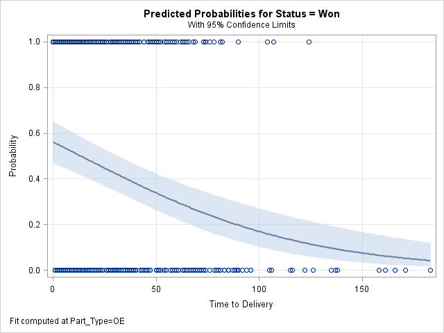
Odds-ratio estimate for time_to_delivery is 0.982. This means that every unit increase in delivery time is associated with 0.018=1.8% decrease in odds of winning the deal. We can see this effect via EFFECTPLOT FIT statement:

							
								PROC LOGISTIC DATA = tutorial.lostsales;

								CLASS status part_type;

								MODEL status = time_to_delivery part_type / LACKFIT;

								EFFECTPLOT FIT(X=time_to_delivery);

								RUN;

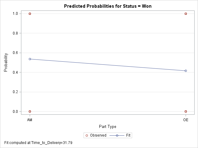
As to the part_type, 1.609 means that odds for sales of AM are 1.609 times the odds of sales of OE. We can see this with EFFECTPLOT INTERACTION statement:

							
								PROC LOGISTIC DATA = tutorial.lostsales;

								CLASS status part_type;

								MODEL status = time_to_delivery part_type / LACKFIT;

								EFFECTPLOT INTERACTION(X=part_type);

								RUN;