
Sampling
There are a variety of probability sampling strategies. Frequently used probability sampling strategies are simple, systematic, stratified, and cluster sampling. Simple random sampling may be the best known sampling strategy. Systematic random sampling uses a list of population elements. If elements can be assumed to be randomly listed, then a starting point is randomly identified, and elements are selected using a sampling interval. These intervals are calculated by dividing the desired sample size by the number of elements in the sampling frame. For example, to select a sample size of 50 from a sampling frame with 100 elements, pick a random starting point and select every second element until 50 elements are selected. Stratified sampling uses groups to achieve representativeness, or to ensure that a certain number of elements from each group are selected. In a stratified sample, the sampling frame is divided into nonoverlapping groups or strata (e.g., age groups, gender). Then a random sample is taken from each stratum. This technique, for example, can be used to study a small subgroup of a population that could be excluded in a simple random sample. Cluster sampling enables random sampling from either a very large population or one that is geographically diverse. An important objective of cluster sampling is to reduce costs by increasing sampling efficiency. A problem with cluster sampling is that, although every cluster has the same chance of being selected, elements within large clusters have a greatly reduced chance of being selected in the final sample. Using the probability proportionate to size (PPS) technique corrects this error. PPS takes into account the difference in cluster size and adjusts the chance that clusters will be selected. That is, PPS increases the odds that elements in larger clusters will be selected [1]. All of these methods are available with the SURVEYSELECT procedure.
The SURVEYSELECT procedure provides a variety of methods for selecting probability-based random samples. The procedure can select a simple random sample or can sample according to a complex multistage sample design that includes stratification, clustering, and unequal probabilities of selection.
Let's use an imaginary dataset to demonstrate each sampling method. For example let's assume we have dataset that lists number of accidents per each day of a week and we would like to get a sample out of it. A few observations from the dataset looks like this (you can download the full dataset from here.)
| Obs | day | dayofweek | n |
|---|---|---|---|
| 1 | 1 | Monday | 49 |
| 2 | 2 | Tuesday | 30 |
| 3 | 3 | Wednesday | 29 |
| 4 | 4 | Thursday | 53 |
| 5 | 5 | Friday | 73 |
| 6 | 6 | Saturday | 103 |
| 7 | 7 | Sunday | 66 |
| 8 | 8 | Monday | 52 |
| 9 | 9 | Tuesday | 30 |
| 10 | 10 | Wednesday | 28 |
Here's a summary of the original dataset:
| Analysis Variable : n | |||||
|---|---|---|---|---|---|
| dayofweek | N | Mean | Std Dev | Minimum | Maximum |
| Friday | 3000 | 69.54 | 18.37 | 11.00 | 134.00 |
| Monday | 3000 | 59.55 | 9.88 | 20.00 | 91.00 |
| Saturday | 3000 | 79.61 | 17.73 | 4.00 | 142.00 |
| Sunday | 3000 | 59.88 | 13.11 | 19.00 | 103.00 |
| Thursday | 3000 | 54.34 | 8.02 | 28.00 | 83.00 |
| Tuesday | 3000 | 39.61 | 7.13 | 9.00 | 69.00 |
| Wednesday | 3000 | 34.32 | 5.99 | 15.00 | 56.00 |
Simple Random Sampling
The method of simple random sampling without replacement (METHOD=SRS) selects units with equal probability and without replacement and also the default sampling method in SAS. Each possible sample of different units out of has the same probability of being selected. After a unit is selected it cannot be selected again. Here's how we do it in SAS:
								PROC SURVEYSELECT DATA=tutorial.sampling SAMPSIZE=100 METHOD=SRS SEED=1234 OUT=sample;

								RUN;
Here's a summary of our sample:
| Analysis Variable : n | |||||
|---|---|---|---|---|---|
| dayofweek | N | Mean | Std Dev | Minimum | Maximum |
| Friday | 12 | 64.25 | 16.03 | 39.00 | 87.00 |
| Monday | 10 | 54.00 | 8.97 | 44.00 | 75.00 |
| Saturday | 18 | 82.11 | 21.92 | 33.00 | 113.00 |
| Sunday | 18 | 63.44 | 14.20 | 44.00 | 93.00 |
| Thursday | 15 | 54.87 | 7.37 | 43.00 | 65.00 |
| Tuesday | 16 | 42.13 | 7.64 | 26.00 | 53.00 |
| Wednesday | 11 | 33.09 | 6.20 | 24.00 | 42.00 |
The problem with our sample is the distribution of days; clearly Saturday and Sunday are overrepresented whereas Monday and Wednesday are underrepresented. To fix this we have to specify a strata preceded by sorting the data by specified strata (this is one of the things that I still don't get - why this sorting cannot be done by the process itself but has to be separately conducted):
								PROC SORT DATA=tutorial.sampling;

								BY dayofweek;

								RUN;


								PROC SURVEYSELECT DATA=tutorial.sampling SAMPSIZE=14 METHOD=SRS SEED=1234 OUT=sample;

								STRATA dayofweek;

								RUN;
| Analysis Variable : n | |||||
|---|---|---|---|---|---|
| dayofweek | N | Mean | Std Dev | Minimum | Maximum |
| Friday | 14 | 60.71 | 20.41 | 11.00 | 86.00 |
| Monday | 14 | 61,43 | 9.43 | 47.00 | 81.00 |
| Saturday | 14 | 79.07 | 21.83 | 46.00 | 126.00 |
| Sunday | 14 | 65.57 | 13.79 | 38.00 | 83.00 |
| Thursday | 14 | 52.07 | 6.79 | 37.00 | 65.00 |
| Tuesday | 14 | 37.64 | 7.63 | 27.00 | 49.00 |
| Wednesday | 14 | 33.93 | 5.59 | 26.00 | 42.00 |
Note we specified the sample size as 14 for each strata so that we have a sample size of 14x7=98.
Strata option worked well in our example because there are equal number of observations for each day of the week but what if we have a sample with unequal distribution of days of week and we represent this proportion in our sample. Assume for example that our original data looked like this instead:
| Analysis Variable : n | |||||
|---|---|---|---|---|---|
| dayofweek | N | Mean | Std Dev | Minimum | Maximum |
| Friday | 211 | 74.41 | 14.77 | 51.00 | 134.00 |
| Monday | 190 | 63.56 | 7.61 | 51.00 | 86.00 |
| Saturday | 232 | 81.60 | 16.70 | 52.00 | 131.00 |
| Sunday | 162 | 65.74 | 10.06 | 51.00 | 97.00 |
| Thursday | 183 | 58.89 | 5.56 | 51.00 | 73.00 |
| Tuesday | 21 | 53.81 | 2.82 | 51.00 | 59.00 |
| Wednesday | 1 | 52.00 | - | 52.00 | 52.00 |
To get an accurate sample representing the original distribution of days of the week, we can use METHOD=SEQ, sequential random sampling which would take the original distribution into account without a need to specify strata at all. Here's how we do it:
								PROC SURVEYSELECT DATA=tutorial.sampling SAMPSIZE=100 METHOD=SEQ SEED=1234 OUT=sample;

								RUN;
| Analysis Variable : n | |||||
|---|---|---|---|---|---|
| dayofweek | N | Mean | Std Dev | Minimum | Maximum |
| Friday | 21 | 73.24 | 12.07 | 52.00 | 95.00 |
| Monday | 19 | 62.47 | 6.10 | 51.00 | 73.00 |
| Saturday | 23 | 80.00 | 15.37 | 56.00 | 110.00 |
| Sunday | 16 | 63.94 | 11.11 | 51.00 | 97.00 |
| Thursday | 19 | 58.42 | 5.68 | 52.00 | 69.00 |
| Tuesday | 2 | 55.00 | 4.24 | 52.00 | 58.00 |
If we instead want to create a sample with replacement instead, we should use METHOD=URS (unrestricted random sampling). With replacement in place of course, there is always a chance of selecting the same observation more than once. By default SAS removes duplicate observations from the final dataset. Let's demonstrate this with an example:
								PROC SURVEYSELECT DATA=tutorial.sampling SAMPSIZE=14 METHOD=URS SEED=4345 OUT=sample;

								STRATA dayofweek;

								RUN;
| Analysis Variable : n | |||||
|---|---|---|---|---|---|
| dayofweek | N | Mean | Std Dev | Minimum | Maximum |
| Friday | 14 | 65.50 | 18.10 | 26.00 | 91.00 |
| Monday | 14 | 62.79 | 9.01 | 44.00 | 77.00 |
| Saturday | 14 | 86.71 | 23.31 | 45.00 | 132.00 |
| Sunday | 14 | 59.36 | 12.24 | 40.00 | 79.00 |
| Thursday | 13 | 55.15 | 5.15 | 46.00 | 63.00 |
| Tuesday | 14 | 40.07 | 5.31 | 32.00 | 47.00 |
| Wednesday | 14 | 32.50 | 5.84 | 19.00 | 42.00 |
As can be seen, we have 13 observations for Thursday instead of 14 we specified. In order to keep the duplicate instead we add OUTHITS option to our code.
								PROC SURVEYSELECT DATA=tutorial.sampling SAMPSIZE=14 METHOD=URS OUTHITS SEED=4345 OUT=sample;

								STRATA dayofweek;

								RUN;
| Analysis Variable : n | |||||
|---|---|---|---|---|---|
| dayofweek | N | Mean | Std Dev | Minimum | Maximum |
| Friday | 14 | 65.50 | 18.10 | 26.00 | 91.00 |
| Monday | 14 | 62.79 | 9.01 | 44.00 | 77.00 |
| Saturday | 14 | 86.71 | 23.31 | 45.00 | 132.00 |
| Sunday | 14 | 59.36 | 12.24 | 40.00 | 79.00 |
| Thursday | 14 | 55.21 | 4.95 | 46.00 | 63.00 |
| Tuesday | 14 | 40.07 | 5.31 | 32.00 | 47.00 |
| Wednesday | 14 | 32.50 | 5.84 | 19.00 | 42.00 |
Example: Titanic Passengers
Description: TThe sinking of the RMS Titanic is one of the most infamous shipwrecks in history. On April 15, 1912, during her maiden voyage, the Titanic sank after colliding with an iceberg, killing 1502 out of 2224 passengers and crew. This data table describes the survival status of 1309 of the 1324 individual passengers on the Titanic. Information on the 899 crew members is not included
name: Passenger name.
survived: Yes or No.
passenger_class: 1, 2, or 3 corresponding to 1st, 2nd, or 3rd class.
sex: Passenger sex.
age: Passenger age.
siblings_and_spouses: The number of siblings and spouses aboard.
parents_and_children: The number of parents and children aboard.
fare: The passenger fare.
port: Port of embarkment (C = Cherbourg; Q = Queenstown; S = Southampton).
home_dest: The home or final intended destination of the passenger.
Source: Building Better Models with JMP Pro
Download the data from here
Task: Create a data set with %70 train and 30% test, derive a logistic regression model to find factors effecting survival chance with train data and test it with test data.
Let's first create our test and train dataset with SURVEYSELECT procedure:
								PROC SURVEYSELECT DATA=tutorial.titanic RATE=0.3 OUTALL METHOD=SRS SEED=1234 OUT=sample;

								RUN;
RATE defines the percent of data to be selected - 30% in our case.
OUTALL tells SAS to output not just the selected but also unselected data in the output. To separate the selected from unselected, SAS will create a column called "selected" with value 1 for selected and 0 for unselected.
METHOD=SRS specifies the selection method = sampling with replacement in this case. Other option is URS.
SEED=1234 is simply a seed number for generating random selection. This can be any number. If you use the same number you will get the same result - it's good for reproducibility.
Now we have a new dataset with a "selected" column and we would like to create two datasets with names titanic_train and titanic_test. To do this we use DATA procedure:
								DATA titanic_train titanic_test;

								SET sample;

								IF selected=0 THEN OUTPUT titanic_train;

								ELSE OUTPUT titanic_test;
Next we can run our first logistic regression model with train data:
								PROC LOGISTIC DATA= titanic_train;

								CLASS survived passenger_class sex port;

								MODEL survived = passenger_class sex port age siblings_and_spouses parents_and_children fare;

								RUN;
| Model Fit Statistics | ||
|---|---|---|
| Criterion | Intercept Only | Intercept and Covariates |
| AIC | 977.400 | 682.571 |
| SC | 981.984 | 728.405 |
| -2 Log L | 975.400 | 662.571 |
| Testing Global Null Hypothesis: BETA=0 | |||
|---|---|---|---|
| Test | Chi-Square | DF | Pr > ChiSq |
| Likelihood Ratio | 312.8295 | 9 | <.0001 |
| Score | 272.0024 | 9 | <.0001 |
| Wald | 187.3937 | 9 | <.0001 |
| Type 3 Analysis of Effects | |||
|---|---|---|---|
| Effect | DF | Wald Chi-Square |
Pr > ChiSq |
| Passenger_Class | 2 | 39.9014 | <.0001 |
| Sex | 1 | 129.7333 | <.0001 |
| Port | 2 | 22.1606 | <.0001 |
| Age | 1 | 24.2463 | <.0001 |
| Siblings_and_Spouses | 1 | 7.5274 | 0.0061 |
| Parents_and_Children | 1 | 0.0452 | 0.8316 |
| Fare | 1 | 0.0014 | 0.9697 |
| Analysis of Maximum Likelihood Estimates | ||||||
|---|---|---|---|---|---|---|
| Parameter | DF | Estimate | Standard Error |
Wald Chi-Square |
Pr > ChiSq | |
| Intercept | 1 | 1.0919 | 0.3459 | 9.9635 | 0.0016 | |
| Passenger_Class | 1 | 1 | 0.9339 | 0.2050 | 20.7613 | <.0001 |
| Passenger_Class | 2 | 1 | 0.0812 | 0.1562 | 0.2699 | 0.6034 |
| Sex | female | 1 | 1.2423 | 0.1091 | 129.7333 | <.0001 |
| Port | C | 1 | 1.1380 | 0.2474 | 21.1600 | <.0001 |
| Port | Q | 1 | -1.2993 | 0.3786 | 11.7762 | 0.0006 |
| Age | 1 | -0.0394 | 0.00800 | 24.2463 | <.0001 | |
| Siblings_and_Spouses | 1 | -0.3617 | 0.1318 | 7.5274 | 0.0061 | |
| Parents_and_Children | 1 | 0.0260 | 0.1223 | 0.0452 | 0.8316 | |
| Fare | 1 | 0.000099 | 0.00260 | 0.0014 | 0.9697 | |
| Odds Ratio Estimates | |||
|---|---|---|---|
| Effect | Point Estimate | 95% Wald Confidence Limits |
|
| Passenger_Class 1 vs 3 | 7.022 | 3.648 | 13.516 |
| Passenger_Class 2 vs 3 | 2.993 | 1.861 | 4.814 |
| Sex female vs male | 11.997 | 7.823 | 18.397 |
| Port C vs S | 2.655 | 1.600 | 4.406 |
| Port Q vs S | 0.232 | 0.077 | 0.695 |
| Age | 0.961 | 0.946 | 0.977 |
| Siblings_and_Spouses | 0.696 | 0.538 | 0.902 |
| Parents_and_Children | 1.026 | 0.808 | 1.304 |
| Fare | 1.000 | 0.995 | 1.005 |
| Association of Predicted Probabilities and Observed Responses |
|||
|---|---|---|---|
| Percent Concordant | 84.8 | Somers' D | 0.697 |
| Percent Discordant | 15.1 | Gamma | 0.697 |
| Percent Tied | 0.0 | Tau-a | 0.336 |
| Pairs | 125852 | c | 0.849 |
Variables parents_and_children and fare are relevant so we will remove them from our model. Also we will add a new option to PROC LOGISTIC statement: OUTMODEL=titanic. This will save the model (formula) for making estimations on the test data set.
								PROC LOGISTIC DATA=titanic_train OUTMODEL=titanic;

								CLASS survived passenger_class sex port;

								MODEL survived = passenger_class sex port age siblings_and_spouses;

								RUN;
| Model Fit Statistics | ||
|---|---|---|
| Criterion | Intercept Only | Intercept and Covariates |
| AIC | 978.434 | 678.689 |
| SC | 983.019 | 715.367 |
| -2 Log L | 976.434 | 662.689 |
| Testing Global Null Hypothesis: BETA=0 | |||
|---|---|---|---|
| Test | Chi-Square | DF | Pr > ChiSq |
| Likelihood Ratio | 313.7450 | 7 | <.0001 |
| Score | 272.7190 | 7 | <.0001 |
| Wald | 187.6911 | 7 | <.0001 |
| Type 3 Analysis of Effects | |||
|---|---|---|---|
| Effect | DF | Wald Chi-Square |
Pr > ChiSq |
| Passenger_Class | 2 | 52.2370 | <.0001 |
| Sex | 1 | 137.4998 | <.0001 |
| Port | 2 | 22.5883 | <.0001 |
| Age | 1 | 24.6579 | <.0001 |
| Siblings_and_Spouses | 1 | 8.0404 | 0.0046 |
| Analysis of Maximum Likelihood Estimates | ||||||
|---|---|---|---|---|---|---|
| Parameter | DF | Estimate | Standard Error |
Wald Chi-Square |
Pr > ChiSq | |
| Intercept | 1 | 1.1068 | 0.3281 | 11.3792 | 0.0007 | |
| Passenger_Class | 1 | 1 | 0.9380 | 0.1743 | 28.9742 | <.0001 |
| Passenger_Class | 2 | 1 | 0.0795 | 0.1516 | 0.2746 | 0.6002 |
| Sex | female | 1 | 1.2482 | 0.1064 | 137.4998 | <.0001 |
| Port | C | 1 | 1.1421 | 0.2463 | 21.5095 | <.0001 |
| Port | Q | 1 | -1.3050 | 0.3781 | 11.9122 | 0.0006 |
| Age | 1 | -0.0395 | 0.00796 | 24.6579 | <.0001 | |
| Siblings_and_Spouses | 1 | -0.3523 | 0.1242 | 8.0404 | 0.0046 | |
| Odds Ratio Estimates | |||
|---|---|---|---|
| Effect | Point Estimate | 95% Wald Confidence Limits |
|
| Passenger_Class 1 vs 3 | 7.067 | 4.062 | 12.296 |
| Passenger_Class 2 vs 3 | 2.995 | 1.870 | 4.796 |
| Sex female vs male | 12.138 | 7.997 | 18.424 |
| Port C vs S | 2.663 | 1.611 | 4.399 |
| Port Q vs S | 0.230 | 0.077 | 0.689 |
| Age | 0.961 | 0.946 | 0.976 |
| Siblings_and_Spouses | 0.703 | 0.551 | 0.897 |
| Association of Predicted Probabilities and Observed Responses |
|||
|---|---|---|---|
| Percent Concordant | 84.9 | Somers' D | 0.698 |
| Percent Discordant | 15.0 | Gamma | 0.699 |
| Percent Tied | 0.1 | Tau-a | 0.337 |
| Pairs | 126144 | c | 0.849 |
Let's now see how good our model is with our test data set.
								PROC LOGISTIC INMODEL=titanic;

								SCORE DATA=titanic_test OUT=titanic_score FITSTAT ;

								RUN;
| Fit Statistics for SCORE Data | |||||||||||
|---|---|---|---|---|---|---|---|---|---|---|---|
| Data Set | Total Frequency | Log Likelihood | Error Rate | AIC | AICC | BIC | SC | R-Square | Max-Rescaled R-Square |
AUC | Brier Score |
| WORK.TITANIC_TEST | 320 | -150.1 | 0.2000 | 316.1415 | 316.6046 | 346.2881 | 346.2881 | 0.342782 | 0.461507 | 0.846468 | 0.148635 |
Our error rate is 20%, not bad. Another measure I typically look into is Brier Score. Brier Score is the mean squared difference between the predicted probability and the actual outcome. The lower the Brier score is, the better our model is. A Brier score of zero means perfect fit and one means worst fit possible. For our case it's 0.15, not so bad - not amazing either. If we had randomly estimated survival, our Brier score would have been around 0.25, so 0.15 is not too bad.
When saving scores, SAS puts two columns in the output: f_survived and i_survived for each observation. f_survived is the value of survived in the titanic_test dataset and i_survived is the estimated value of the survival based on the logistic model. Therefore the more agreeement between these columns, the better our model is. We can utilize PROC FREQ to see how good our estimates are:
								PROC FREQ DATA=titanic_score;

								TABLE f_survived*i_survived / AGREE;

								RUN;
And here is our output:
| McNemar's Test | |
|---|---|
| Statistic (S) | 1.5625 |
| DF | 1 |
| Pr > S | 0.2113 |
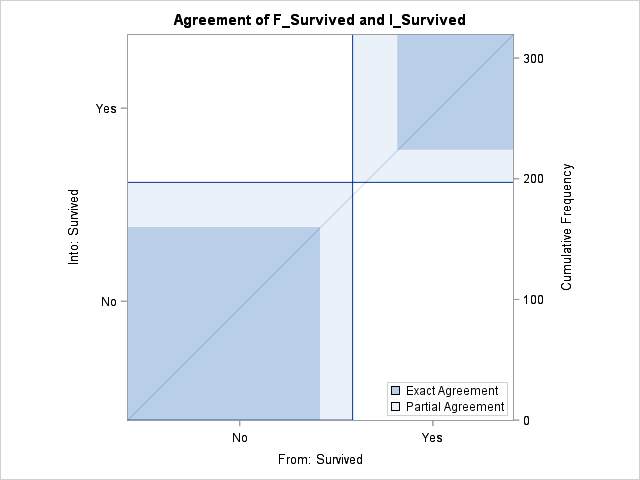
p-value for McNemar test is 0.2113. Higher p-values mean better agreement. We can use this measure to compare different models. Agree plot shows our fit visually. Note that this measure would only be useful for relatively balanced designs.
Preventing Bias in Sampling
It is important to create samples that represent original data accurately otherwise we would have a biased sample. For example, take a look at the carddefault data which shows the credit card defaults with other socio-economic variables. A predictive model would try to estimate the defaulting. Let's take a look at the default and student ratios in the dataset via PROC FREQ:
								PROC FREQ DATA=tutorial.carddefault;

								TABLES default student;

								RUN;
| default | Frequency | Percent | Cumulative Frequency |
Cumulative Percent |
|---|---|---|---|---|
| No | 9667 | 96.67 | 9667 | 96.67 |
| Yes | 333 | 3.33 | 10000 | 100.00 |
| student | Frequency | Percent | Cumulative Frequency |
Cumulative Percent |
|---|---|---|---|---|
| No | 7056 | 70.56 | 7056 | 70.56 |
| Yes | 2944 | 29.44 | 10000 | 100.00 |
Now let's create a training sample from our dataset via PROC SURVEYSELECT and see the distribution via PROC FREQ:
								PROC SURVEYSELECT DATA=tutorial.carddefault OUT=train_carddefault RATE=0.7 SEED=1234;

								RUN;


								PROC FREQ DATA=train_carddefault;

								TABLES default student;

								RUN;
| default | Frequency | Percent | Cumulative Frequency |
Cumulative Percent |
|---|---|---|---|---|
| No | 6742 | 96.31 | 6742 | 96.31 |
| Yes | 258 | 3.69 | 7000 | 100.00 |
| student | Frequency | Percent | Cumulative Frequency |
Cumulative Percent |
|---|---|---|---|---|
| No | 4969 | 70.99 | 4969 | 70.99 |
| Yes | 2031 | 29.01 | 7000 | 100.00 |
As can be seen from above default=Yes is oversampled and student=Yes is undersampled. To remedy this we have to use STRATA statement with PROC SURVEYSELECT. Note that sorting the data is required before invoking STRATA.
								PROC SORT DATA=tutorial.carddefault;

								BY default student;

								RUN;


								PROC SURVEYSELECT DATA=tutorial.carddefault OUT=train_carddefault RATE=0.7 SEED=1234;

								STRATA default student;

								RUN;


								PROC FREQ DATA=train_carddefault;

								TABLES default student;

								RUN;
| default | Frequency | Percent | Cumulative Frequency |
Cumulative Percent |
|---|---|---|---|---|
| No | 6767 | 96.66 | 6767 | 96.66 |
| Yes | 234 | 3.34 | 7001 | 100.00 |
| student | Frequency | Percent | Cumulative Frequency |
Cumulative Percent |
|---|---|---|---|---|
| No | 4940 | 70.56 | 4940 | 70.56 |
| Yes | 2061 | 29.44 | 7001 | 100.00 |
- Determining Sample Size: Balancing Power, Precision, and Practicality, P. Dattalo

Lrrr
Senior blog writer
Lrrr, ruler of the planet Omicron Persei 8, is a middle-aged Omicronian man with a bad temper and soft spots for the conquering of planets and 20th century television.
Popular Posts

Space The Final Frontier
02 Hours ago

The Amazing Hubble
02 Hours ago

Astronomy Or Astrology
02 Hours ago

Asteroids telescope
02 Hours ago

Leave a Comment