
Random Forest
Random forests or random decision forests are an ensemble learning method for classification, regression and other tasks that operates by constructing a multitude of decision trees at training time and outputting the class that is the mode of the classes (classification) or mean prediction (regression) of the individual trees. Random decision forests correct for decision trees' habit of overfitting to their training set. One of the most attractive feature of random forests (and decision trees) is its robustness to outliers. SAS procedure for implementing random forest models is PROC HPFOREST.
Example: Titanic Passengers
We used this data set in Lecture 20 to derive a logistic regression model to estimate the survival of a passenger from several variables. Here we will use random forest method to do the same for the same data set.
Once again let's create our test and train dataset with SURVEYSELECT procedure (you can see the details in Lecture 20):
								PROC SURVEYSELECT DATA=tutorial.titanic RATE=0.3 OUTALL METHOD=SRS SEED=1234 OUT=sample;

								RUN;


								DATA titanic_train titanic_test;

								SET sample;

								IF selected=0 THEN OUTPUT titanic_train;

								ELSE OUTPUT titanic_test;
Here is the code for our random forest model:
								PROC HPFOREST DATA=titanic_train MAXTREES=20 ALPHA=1 SEED=9999 MAXDEPTH=20 VARS_TO_TRY=5 LEAFSIZE=3;

								TARGET survived / LEVEL=BINARY;

								INPUT sex / LEVEL=BINARY;

								INPUT port passenger_class / LEVEL=NOMINAL;

								INPUT age siblings_and_spouses parents_and_children fare / LEVEL=INTERVAL;

								SAVE FILE="D:\titanic.bin";

								RUN;
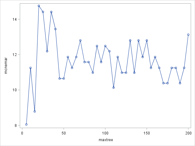
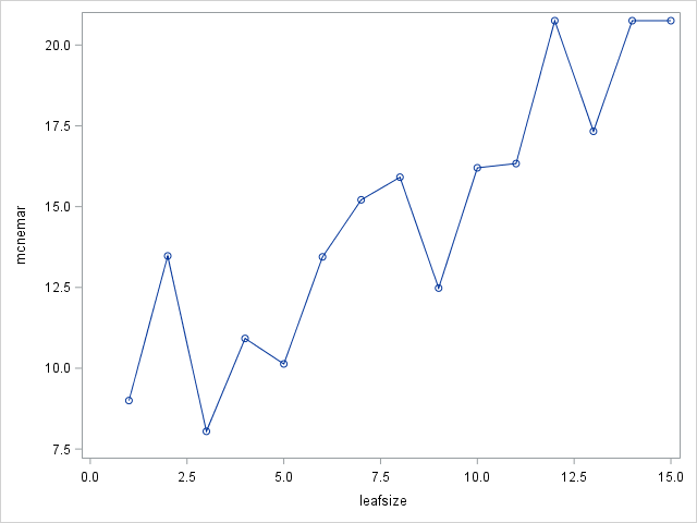
MAXTREES specifies the number of trees in the forest. n is a positive integer. The default value of n is 100. Higher numbers take more time to calculate. You can think of this as similar to "number of iterations": once you reach a plateau, higher numbers won't improve the result. You don't have to specify this and default works just well most of the times. Below graph shows the McNemar's value with different MAXTREE numbers. It can be seen that a plateau is reached around 50 - increasing the number of trees won't make a difference. Note that the lower tree values seem to have lower McNemar value however this is misleading. I suggest not to set number of trees below 50.
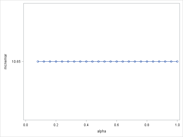
ALPHA specifies a threshold p-value for the significance level of a test of association of a candidate variable with the target. If no association meets this threshold, the node is not split. The default value is 1. Effect of ALPHA in our case is shown below.
SEED specifies the seed for generating random numbers. It's a good idea to specify this number so that you can reproduce your results. It can be any number.
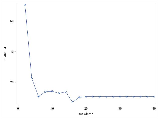
MAXDEPTH specifies the maximum depth of a node in any tree that PROC HPFOREST creates. The depth of a node equals the number of splitting rules needed to define the node. The root node has depth 0. The children of the root have depth 1, the children of those children have depth 2, and so on. The smallest acceptable value of d is 1. The default value of d is 20 (implying a maximum of 1,048,576 leaves).
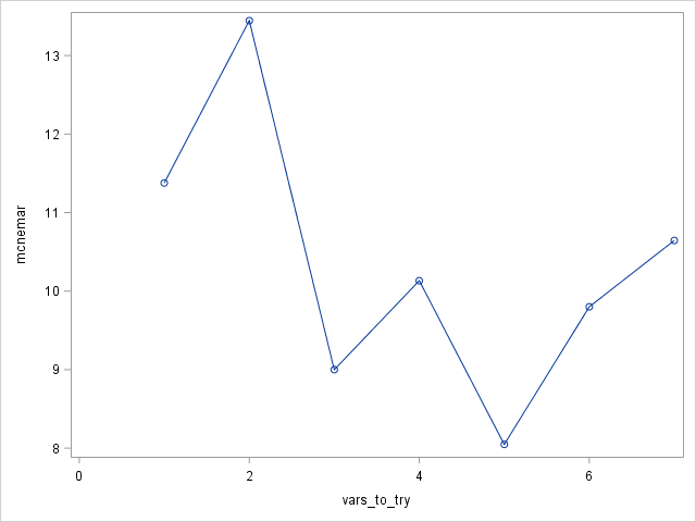
VARS_TO_TRY specifies the number of input variables to consider splitting on in a node. m ranges from 1 to the number of input variables, v. The default value of m is square root of v . Specify VARS_TO_TRY=ALL to use all the inputs as candidates in a node. I set this value to 5 since we found earlier in our logistic regression model that 2 of the 7 variables were irrelevant.
LEAFSIZE specifies the smallest number of training observations a new branch can have. Default value is 1.
To test our generated model with our test data set, we use HP4SCORE procedure. Remember the model file we saved (titanic.bin) earlier with the HPFOREST procedure; we will use this file as input to PROC HP4SCORE and get a score output named titanic_score2.
								PROC HP4SCORE DATA=titanic_test;

								SCORE FILE="D:\titanic.bin" OUT=titanic_score2;

								RUN;
Let's see how our new score output with PROC PRINT:
								PROC PRINT DATA=titanic_score2 (OBS=5);

								RUN;
| Obs | Survived | P_SurvivedNO | P_SurvivedYES | I_Survived | _WARN_ |
|---|---|---|---|---|---|
| 1 | No | 0.55583 | 0.44417 | NO | |
| 2 | Yes | 0.78528 | 0.21472 | NO | |
| 3 | Yes | 0.02667 | 0.97333 | YES | |
| 4 | Yes | 0.05167 | 0.94833 | YES | |
| 5 | Yes | 0.00000 | 1.00000 | YES |
We need to standardize this table so that it will be identical to our previous table from logistic regression scoring. To do this we use DATA step:
								DATA titanic_score2;

								SET titanic_score2 (RENAME=(survived=f_survived);

								IF i_survived="YES" THEN i_survived="Yes";

								ELSE IF i_survived="NO" THEN i_survived="No";

								DROP p_survivedno p_survivedyes _warn_;


								PROC PRINT DATA=titanic_score2 (OBS=5);

								RUN;
Now our table looks OK:
| Obs | f_survived | I_Survived |
|---|---|---|
| 1 | No | No |
| 2 | Yes | No |
| 3 | Yes | Yes |
| 4 | Yes | Yes |
| 5 | Yes | Yes |
Let's run PROC FREQ:
								PROC FREQ DATA=titanic_score2;

								TABLE f_survived*i_survived / AGREE;

								RUN;
| McNemar's Test | |
|---|---|
| Statistic (S) | 5.9024 |
| DF | 1 |
| Pr > S | 0.0151 |
p-value for McNemar's test is 0.0151, way lower than that of obtained through logistic regression (0.2113). Therefore our logistic regression model is better than random forest model for the titanic data set.
Example: Credit Card Marketing
Description: A bank would like to understand the demographics and other characteristics associated with whether a customer accepts a credit card offer. Observational data is somewhat limited for this kind of problem, in that often the company sees only those who respond to an offer. To get around this, the bank designs a focused marketing study, with 18,000 current bank customers. This focused approach allows the bank to know who does and does not respond to the offer, and to use existing demographic data that is already available on each customer.
Each customer receives an offer for a new credit card that has a particular type of reward program associated with it. The type of mailing is varied, with some customers receiving a letter and others receiving postcards. The reward type and mailing type are varied in a balanced random fashion across the prospective customer demographics. After a set period of time, whether the individual has responded positively to the mailer and has opened a new credit card account is recorded.
id: Customer ID.
accepted: Whether customer accepted the offer or not (Yes/No).
reward: Type of reward offered.
type: Letter or postcard.
income: Low, Medium or High.
accounts: Number of non-credit card accounts are held by the customer.
overdraft: Customer has overdraft protection or not.
creditrate: Credit rating of the customer: Low, Medium or High.
cards: Number of credit cards held at the bank by the customer.
homes: Number of homes owned by the customer.
household: Number of individuals in the family.
ownhome: Customer owns their home or not.
avgbalance: Average account balance of the customer.
q1balance: Average balance for Q1 in the last year.
q2balance: Average balance for Q2 in the last year.
q3balance: Average balance for Q3 in the last year.
q4balance: Average balance for Q4 in the last year.
Source: Building Better Models With JMP Pro, Grayson et al.
Download the data from here
Task: Design a model for estimating card offer acceptance by a customer.
Let's first start with separating our data into train and test sets with SURVEYSELECT:
								PROC SURVEYSELECT DATA=tutorial.cardoffer RATE=0.3 OUTALL METHOD=SRS SEED=1234 OUT=cardoffer;

								RUN;


								DATA cardoffer_train cardoffer_test;

								SET cardoffer;

								IF selected=0 THEN OUTPUT cardoffer_train;

								ELSE OUTPUT cardoffer_test;
Now that we have the train set ready, we can invoke HPFOREST procedure and see the outcome with HP4SCORE and PROC FREQ:
								PROC HPFOREST DATA=cardoffer_train SEED=9999 ;

								TARGET accepted / LEVEL=BINARY;

								INPUT reward / LEVEL=NOMINAL;

								INPUT type overdraft ownhome / LEVEL=BINARY;

								INPUT income creditrate / LEVEL=ORDINAL;

								INPUT accounts cards homes household q1balance q2balance q3balance q4balance / LEVEL=INTERVAL;

								SAVE FILE="D:\cardoffer.bin";

								RUN;


								PROC HP4SCORE DATA=cardoffer_test;

								SCORE FILE="D:\cardoffer.bin" OUT=score_card;

								RUN;


								PROC FREQ DATA=score_card;

								TABLE accepted*i_accepted / AGREE;

								RUN;
| Table of accepted by I_accepted | ||||||
|---|---|---|---|---|---|---|
| accepted(Offer Accepted) |
I_accepted(Into: accepted) | |||||
| NO | YES | Total | ||||
| No |
|
|
|
|||
| Yes |
|
|
|
|||
| Total |
|
|
|
|||
As you can notice there are only a handful predictions of 'Yes'. This is because the design is unbalanced, i.e. Yes/No rate in the data is a small number. This is normal.

Lrrr
Senior blog writer
Lrrr, ruler of the planet Omicron Persei 8, is a middle-aged Omicronian man with a bad temper and soft spots for the conquering of planets and 20th century television.
Popular Posts

Space The Final Frontier
02 Hours ago

The Amazing Hubble
02 Hours ago

Astronomy Or Astrology
02 Hours ago

Asteroids telescope
02 Hours ago

Leave a Comment