Overdispersion
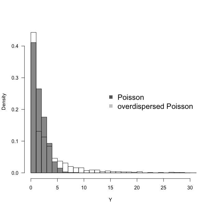
In statistics, overdispersion is the presence of greater variability (statistical dispersion) in a data set than would be expected based on a given statistical model. Overdispersion is often encountered when fitting very simple parametric models, such as those based on the Poisson distribution and this will usually lead to inflated Type I error rates. The Poisson distribution has one free parameter and does not allow for the variance to be adjusted independently of the mean. The choice of a distribution from the Poisson family is often dictated by the nature of the empirical data. For example, Poisson regression analysis is commonly used to model count data. If overdispersion is a feature, an alternative model with additional free parameters may provide a better fit. In the case of count data, a Poisson mixture model like the negative binomial distribution can be proposed instead, in which the mean of the Poisson distribution can itself be thought of as a random variable drawn – in this case – from the gamma distribution thereby introducing an additional free parameter (note the resulting negative binomial distribution is completely characterized by two parameters).
Example: Extramarital Affairs
Description: Data set includes various social and marital factors along with the count of extramarital affairs for 600 people.
naffairs: Number of affairs within last year.
kids: 1=have children 0=no children.
vryunhap: Very unhappily married (1/0).
unhap: Unhappily married (1/0).
avgmarr: Average married (1/0).
hapavg: Happily married (1.0).
vryhap: Very happily married (1/0).
antirel: Anti-religious (1/0)
notrel: Not religious (1/0).
slghtrel: Slightly religious (1/0).
smerel: Somewhat religious (1/0).
vryrel: Very religious (1/0).
yrsmarr1: Year of marriage > 0.75 yrs (1/0).
yrsmarr2: Year of marriage > 1.5 yrs (1/0).
yrsmarr3: Year of marriage > 4.0 yrs (1/0).
yrsmarr4: Year of marriage > 7.0 yrs (1/0).
yrsmarr5: Year of marriage > 10.0 yrs (1/0).
yrsmarr6: Year of marriage > 15.0 yrs (1/0).
Source: https://vincentarelbundock.github.io/Rdatasets/doc/COUNT/affairs.html
Download the data from here
Task: Design a model for estimating number of affairs.
Let's try PROC GENMOD with poisson distribution option:
								PROC GENMOD DATA=tutorial.affairs;

								CLASS kids--yrsmarr6;

								MODEL naffairs = kids--yrsmarr6 / DIST=POISSON;

								RUN;
| Criteria For Assessing Goodness Of Fit | |||
|---|---|---|---|
| Criterion | DF | Value | Value/DF |
| Deviance | 586 | 2303.1626 | 3.9303 |
| Scaled Deviance | 586 | 2303.1626 | 3.9303 |
| Pearson Chi-Square | 586 | 4050.5305 | 6.9122 |
| Scaled Pearson X2 | 586 | 4050.5305 | 6.9122 |
| Log Likelihood | -235.1784 | ||
| Full Log Likelihood | -1398.5763 | ||
| AIC (smaller is better) | 2827.1525 | ||
| AICC (smaller is better) | 2827.9730 | ||
| BIC (smaller is better) | 2893.1314 | ||
‘Criteria For Assessing Goodness Of Fit’ section of output suggests that, because value/df for both deviance and Pearson Chi-Square statistics is much higher than 1, Poisson model is not quite adequate to describe the counts of hypotensions and crampings. It also suggests that there is overdispersion.
Negative-binomial distribution is a benchmark model to account for overdisperion on count responses. We can test for overdispersion in a Poisson model by using the DIST=NEGBIN, SCALE=0, and NOSCALE options in the MODEL statement of PROC GENMOD. When used together, these options test whether overdispersion of the form μ+kμ2 exists by testing whether the negative binomial dispersion parameter, k, is zero. When k=0, the negative binomial distribution is equivalent to the Poisson distribution. Let's test whether there is overdispersion in our data.
								PROC GENMOD DATA=tutorial.affairs;

								CLASS kids--yrsmarr6;

								MODEL naffairs = kids--yrsmarr6 / DIST=NEGBIN SCALE=0 NOSCALE;

								RUN;
| Lagrange Multiplier Statistics | |||
|---|---|---|---|
| Parameter | Chi-Square | Pr > ChiSq | |
| Dispersion | 259.7461 | <.0001 | * |
| * One-sided p-value | |||
Our suspicions were correct; there is overdispersion. There are various distributions to implement instead of Poisson:
- Negative binomial
- Zero-inflated poisson
- Zero-inflated negative binomial
- Hurdle poisson
- Hurdle negative binomial
- Generalized poisson
								PROC GENMOD DATA=tutorial.affairs;

								CLASS kids--yrsmarr6;

								MODEL naffairs = kids--yrsmarr6 / DIST=POISSON DSCALE;

								RUN;
| Criteria For Assessing Goodness Of Fit | |||
|---|---|---|---|
| Criterion | DF | Value | Value/DF |
| Deviance | 586 | 2303.1626 | 3.9303 |
| Scaled Deviance | 586 | 586.000 | 1.000 |
| Pearson Chi-Square | 586 | 4050.5305 | 6.9122 |
| Scaled Pearson X2 | 586 | 1030.5876 | 1.7587 |
| Log Likelihood | -59.8371 | ||
| Full Log Likelihood | -1398.5763 | ||
| AIC (smaller is better) | 2827.1525 | ||
| AICC (smaller is better) | 2827.9730 | ||
| BIC (smaller is better) | 2893.1314 | ||
Scaled Pearson X2 is still well above 1, therefore we will try negative binomial distribution next:
								PROC GENMOD DATA=tutorial.affairs;

								CLASS kids--yrsmarr6;

								MODEL naffairs = kids--yrsmarr6 / DIST=NEGBIN;

								RUN;
| Criteria For Assessing Goodness Of Fit | |||
|---|---|---|---|
| Criterion | DF | Value | Value/DF |
| Deviance | 586 | 339.8629 | 0.5800 |
| Scaled Deviance | 586 | 339.8629 | 0.5800 |
| Pearson Chi-Square | 586 | 566.8541 | 0.9673 |
| Scaled Pearson X2 | 586 | 566.8541 | 0.9673 |
| Log Likelihood | 439.3546 | ||
| Full Log Likelihood | -724.0433 | ||
| AIC (smaller is better) | 1480.0865 | ||
| AICC (smaller is better) | 1481.0180 | ||
| BIC (smaller is better) | 1550.4640 | ||
Parameter estimates (not shown) tells us that only unhap, antirel, notrel, slghtrel, yrsmarr1, yrsmarr2, yrsmarr3 are significant. We run our model with only these variables:
								PROC GENMOD DATA=tutorial.affairs;

								CLASS kids--yrsmarr6;

								MODEL naffairs = unhap antirel notrel slghtrel yrsmarr1 yrsmarr2 yrsmarr3 / DIST=NEGBIN;

								RUN;
| Criteria For Assessing Goodness Of Fit | |||
|---|---|---|---|
| Criterion | DF | Value | Value/DF |
| Deviance | 593 | 338.5604 | 0.5709 |
| Scaled Deviance | 593 | 338.5604 | 0.5709 |
| Pearson Chi-Square | 593 | 530.2979 | 0.8943 |
| Scaled Pearson X2 | 593 | 530.2979 | 0.8943 |
| Log Likelihood | 435.7320 | ||
| Full Log Likelihood | -727.6659 | ||
| AIC (smaller is better) | 1473.3317 | ||
| AICC (smaller is better) | 1473.6363 | ||
| BIC (smaller is better) | 1512.9191 | ||
| Algorithm converged. |
| Analysis Of Maximum Likelihood Parameter Estimates | ||||||||
|---|---|---|---|---|---|---|---|---|
| Parameter | DF | Estimate | Standard Error |
Wald 95% Confidence Limits | Wald Chi-Square | Pr > ChiSq | ||
| Intercept | 1 | 0.6383 | 0.9363 | -1.1968 | 2.4735 | 0.46 | 0.4954 | |
| unhap | 0 | 1 | -1.0441 | 0.3624 | -1.7544 | -0.3339 | 8.30 | 0.0040 |
| antirel | 0 | 1 | -1.3962 | 0.4489 | -2.2760 | -0.5164 | 9.67 | 0.0019 |
| notrel | 0 | 1 | -1.1257 | 0.3141 | -1.7413 | -0.5101 | 12.85 | 0.0003 |
| slghtrel | 0 | 1 | -1.2156 | 0.3302 | -1.8629 | -0.5683 | 13.55 | 0.0002 |
| yrsmarr1 | 0 | 1 | 1.3507 | 0.4769 | 0.4160 | 2.2853 | 8.02 | 0.0046 |
| yrsmarr2 | 0 | 1 | 1.6580 | 0.3850 | 0.9034 | 2.4126 | 18.54 | <.0001 |
| yrsmarr3 | 0 | 1 | 0.8858 | 0.3404 | 0.2187 | 1.5529 | 6.77 | 0.0093 |
| Dispersion | 1 | 7.0132 | 0.7824 | 5.6358 | 8.7272 | |||
Let's also use SAS graphics to see some of the effects of these parameters. Prior to this we need to reformat the data set and create new columns:
								DATA DATA=tutorial.affairs;

								SET tutorial.affairs;


								IF vryunhap = 1 THEN  happiness = 'Very unhappy';

								ELSE IF unhap = 1 THEN  happiness = 'Unhappy';

								ELSE IF hapavg = 1 THEN  happiness = 'Happy';

								ELSE IF vryhap = 1 THEN  happiness = 'Very happy';

								ELSE IF avgmarr = 1 THEN  happiness = 'Very unhappy';


								IF antirel = 1 THEN  religiosity = 'Anti religious';

								ELSE IF notrel = 1 THEN  religiosity = 'Not religious';

								ELSE IF slghtrel = 1 THEN  religiosity = 'Slightly religious';

								ELSE IF smerel = 1 THEN  religiosity = 'Somewhat religious';

								ELSE IF vryrel = 1 THEN  religiosity = 'Very religious';


								IF yrsmarr1 = 1 THEN  years = '0.75';

								ELSE IF yrsmarr2 = 1 THEN  years = '1.5';

								ELSE IF yrsmarr3 = 1 THEN  years = '4';

								ELSE IF yrsmarr4 = 1 THEN  years = '7';

								ELSE IF yrsmarr5 = 1 THEN  years = '10';

								ELSE IF yrsmarr6 = 1 THEN  years = '15';


								cnt=1;

								RUN;
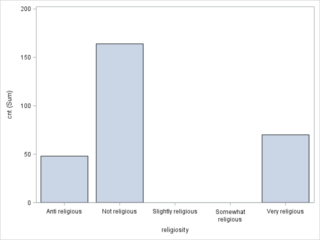
Now let's use a few graphs to understand these variables:
PROC SGPLOT DATA=tutorial.affairs;
VBAR religiosity / RESPONSE=cnt STATSUM;
XAXIS VALUES =('Anti religious' 'Not religious' 'Slightly religious' 'Somewhat religious' 'Very religious');
RUN;
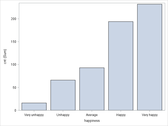
PROC SGPLOT DATA=tutorial.affairs;
VBAR happiness / RESPONSE=cnt STATSUM;
XAXIS VALUES =('Very unhappy' 'Unhappy' 'Average' 'Happy' 'Very happy');
RUN;
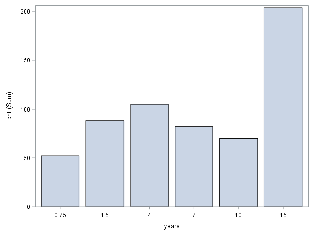
PROC SGPLOT DATA=tutorial.affairs;
VBAR years / RESPONSE=cnt STATSUM;
XAXIS VALUES =('0.75' '1.5' '4' '7' '10' '15');
RUN;

Lrrr
Senior blog writer
Lrrr, ruler of the planet Omicron Persei 8, is a middle-aged Omicronian man with a bad temper and soft spots for the conquering of planets and 20th century television.
Popular Posts

Space The Final Frontier
02 Hours ago

The Amazing Hubble
02 Hours ago

Astronomy Or Astrology
02 Hours ago

Asteroids telescope
02 Hours ago

Leave a Comment