Bayesian Regression with Python

Bayesian Linear Regression

Bayesian linear regression allows a fairly natural mechanism to survive insufficient data, or poor distributed data. It allows you to put a prior on the coefficients and on the noise so that in the absence of data, the priors can take over. More importantly, you can ask Bayesian linear regression which parts (if any) of its fit to the data is it confident about, and which parts are very uncertain (perhaps based entirely on the priors).

One of the important features of Bayesian Regressions is that they can fit quite well with small datasets and next example will demonstrate just that.

Example: Prices of round cut diamonds

Description: A dataset containing the prices and other attributes of almost 54,000 diamonds.

price: Selling price in dollars.
carat: Weight of the diamond.
lot:Area of the houses lot in square feet.
cut: Quality of the cut (Fair, Good, Very Good, Premium, Ideal).
color: Diamond colour, from J (worst) to D (best).
clarity: A measurement of how clear the diamond is (I1 (worst), SI2, SI1, VS2, VS1, VVS2, VVS1, IF (best)).
x: Length in mm.
y: Width in mm.
z: Depth in mm.
depth: Total depth percentage = z / mean(x, y) = 2 * z / (x + y).
table: Width of top of diamond relative to widest point.

Source: https://vincentarelbundock.github.io/Rdatasets/doc/ggplot2/diamonds.html
Download the data from here

Task: Compare Ordinary Linear Regression (OLR) and Bayesian Ridge Regression (BRR) models to estimate price with different sample sizes.

First we will import needed classes and initialize our regression models:

								
									import pandas as pd

									import numpy as np

									import matplotlib.pyplot as plt

									from sklearn.linear_model import LinearRegression, BayesianRidge

									from sklearn.model_selection import train_test_split

									linreg = LinearRegression()

									bayreg = BayesianRidge()

We will score our models by creating train/test samples with test ratio between 0.800 and 0.999 therefore we will have train samples between 0.001*54000 = 54 and 0.200*54000 = 10800 rows. At the end we will have a table like this:

trainsize	linreg_score	bayreg_score
54	0.7	0.7
108	0.8	0.8
162	0.8	0.8
216	0.9	0.9

Let's create our table template:

								
									df = pd.DataFrame(columns=['trainsize', 'linreg_score', 'bayreg_score'])

								
									for i in range(800, 1000, 1):

									    diamonds_train, diamonds_test = train_test_split(diamonds, test_size=i*0.001, random_state=444)

									    linreg.fit(diamonds_train.drop('price', axis=1), diamonds_test.price)

									    bayreg.fit(diamonds_train.drop('price', axis=1), diamonds_test.price)

									    df.loc[i-799,'linreg_score'] = linreg.score(diamonds_test.drop('price', axis=1), diamonds_test.price)

									    df.loc[i-799,'bayreg_score'] = bayreg.score(diamonds_test.drop('price', axis=1), diamonds_test.price)

									    df.loc[i-799,'trainsize'] = np.round((1000-i)*0.001*53940)

Let's see our results with the help of matplotlib

								
									fig = plt.figure(figsize=(15,15))

									ax1 = fig.add_subplot(111)

									ax1.scatter(df.trainsize, df.linreg_score, label='OLR', s=200)

									ax1.scatter(df.trainsize, df.bayreg_score, label='BR', s=200)

									ax1.set_xlim((0,250))

									ax1.set_ylim((0,1))

									ax1.set_xlabel('Training Sample Size', fontsize='large')

									ax1.set_ylabel('Score', fontsize='large')

									ax1.legend(fontsize='x-large')

									fig

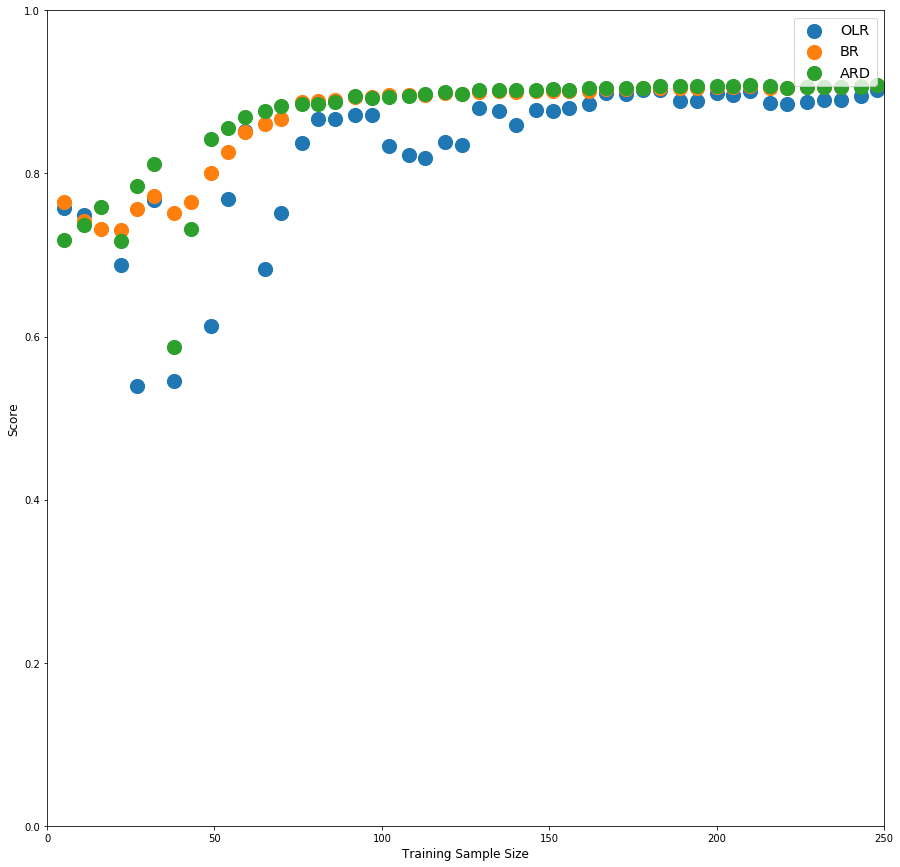
As seen from above Bayesian Ridge performs better when we have limited data for training.

scikit-learn has one more Bayesian regression model type: Automatic Relevance Determination Regression (ARD). Let's also see how this perform the models we tried so far. Note that ARD is much more computationally intensive procedure as opposed to BR and OLR.