Exploratory Statistics II: Frequency Distribution
There are couple of great R packages for descriptive statistics such as skewness and kurtosis, histogram, goodness-of-fit tests, probability plots etc. and we are going to see some of them in this lecture. First, the data set. We will use cake sample data from SAS website. You can download the data from here. This dataset is from a cake-baking contest: each participant's last name, age, score for presentation, score for taste, cake flavor, and number of cake layers. The number of cake layers is missing for two observations. The cake flavor is missing for another observation.
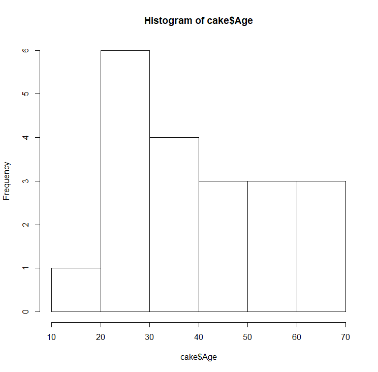
One of the most useful graphs to analyze data is a histogram. A histogram is a plot that lets you discover, and show, the underlying frequency distribution (shape) of a set of continuous data. This allows the inspection of the data for its underlying distribution (e.g., normal distribution), outliers, skewness, etc. We can plot a simple histogram with the hist function:
> hist(cake$Age)
Later we will learn plotting histograms with ggplot2 package which is way more powerful than this simple hist function.
There are couple of functions that helps us to evaluate the normality of a distribution. One of them utilizes Shapiro-Wilk method:
> shapiro.test(cake$Age)
	Shapiro-Wilk normality test

data:  cake$Age
W = 0.93464, p-value = 0.1895
Since p-value > 0.05, Age distribution fit normal distribution. This is the only available normality test with base R (afaik) but nortest package provides a variety of normality tests. One of the tests is Anderson-Darling test:
									> library(nortest)

									> ad.test(cake$Age)
	Anderson-Darling normality test

data:  cake$Age
A = 0.50566, p-value = 0.1785
A-D test agrees with S-W test. Similarly, Cramer von Mises test can be invoked by
> cvm.test(cake$Age)
	Cramer-von Mises normality test

data:  cake$Age
W = 0.080941, p-value = 0.1897
Prev Post
Descriptive Statistics

Lrrr
Senior blog writer
Lrrr, ruler of the planet Omicron Persei 8, is a middle-aged Omicronian man with a bad temper and soft spots for the conquering of planets and 20th century television.
Popular Posts

Space The Final Frontier
02 Hours ago

The Amazing Hubble
02 Hours ago

Astronomy Or Astrology
02 Hours ago

Asteroids telescope
02 Hours ago

Leave a Comment