Exploratory Statistics
First step after data preparation is exploratory statistics. Major SAS procedures to do so are MEANS, UNIVARIATE and FREQ.
PROC MEANS
We will use cake sample data from SAS website. You can download the data from here. This dataset is from a cake-baking contest: each participant's last name, age, score for presentation, score for taste, cake flavor, and number of cake layers. The number of cake layers is missing for two observations. The cake flavor is missing for another observation.
| LastName | Age | PresentScore | TasteScore | Flavor | Layers |
|---|---|---|---|---|---|
| Orlando | 27 | 93 | 80 | Vanilla | 1 |
| Ramey | 32 | 84 | 72 | Rum | 2 |
| Goldston | 46 | 68 | 75 | Vanilla | 1 |
| Roe | 38 | 79 | 73 | Vanilla | 2 |
| Larsen | 23 | 77 | 84 | Chocolate | . |
| Davis | 51 | 86 | 91 | Spice | 3 |
| Strickland | 19 | 82 | 79 | Chocolate | 1 |
| Nguyen | 57 | 77 | 84 | Vanilla | . |
| Hildenbrand | 33 | 81 | 83 | Chocolate | 1 |
| Byron | 62 | 72 | 87 | Vanilla | 2 |
| Sanders | 26 | 56 | 79 | Chocolate | 1 |
| Jaeger | 43 | 66 | 74 | 1 | |
| Davis | 28 | 69 | 75 | Chocolate | 2 |
| Conrad | 69 | 85 | 94 | Vanilla | 1 |
| Walters | 55 | 67 | 72 | Chocolate | 2 |
| Rossburger | 28 | 78 | 81 | Spice | 2 |
| Matthew | 42 | 81 | 92 | Chocolate | 2 |
| Becker | 36 | 62 | 83 | Spice | 2 |
| Anderson | 27 | 87 | 85 | Chocolate | 1 |
| Merritt | 62 | 73 | 84 | Chocolate | 1 |
Let's get the basic statistics from this data by PROC MEANS:


By default PROC MEANS calculates N, Mean, Standard Deviation, Minimum and Maximum for all numerical variables. MAXDEC=2 option limits the number of decimals to 2. To calculate only certain variables, we can state them with a new statement:


PROC MEANS can calculate various statistics other than default ones. To do that we add keywords to the PROC MEANS statement:


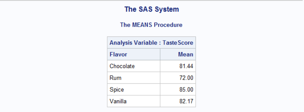
We can also group variables with CLASS statement. Let's say we want to find out average scores for different flavors. Following will achieve that.


Number of observations (N Obs) is printed by default. To omit printing N Obs, we need to use the keyword NONOBS in the PROC MEANS statement:


Output from PROC MEANS can be saved with OUTPUT statement:

Here meanvalues is the name of the output dataset and n, avg and std are the column names for number of observations, mean and standard deviation, respectively.

PROC UNIVARIATE
Our second weapon in SAS arsenal for exploratory statistics is UNIVARIATE procedure. PROC UNIVARIATE provides descriptive statistics such as skewness and kurtosis, histogram, goodness-of-fit tests, probability plots etc. First, the data set. We will use cake sample data from SAS website. You can download the data from here. This dataset is from a cake-baking contest: each participant's last name, age, score for presentation, score for taste, cake flavor, and number of cake layers. The number of cake layers is missing for two observations. The cake flavor is missing for another observation.
| LastName | Age | PresentScore | TasteScore | Flavor | Layers |
|---|---|---|---|---|---|
| Orlando | 27 | 93 | 80 | Vanilla | 1 |
| Ramey | 32 | 84 | 72 | Rum | 2 |
| Goldston | 46 | 68 | 75 | Vanilla | 1 |
| Roe | 38 | 79 | 73 | Vanilla | 2 |
| Larsen | 23 | 77 | 84 | Chocolate | . |
| Davis | 51 | 86 | 91 | Spice | 3 |
| Strickland | 19 | 82 | 79 | Chocolate | 1 |
| Nguyen | 57 | 77 | 84 | Vanilla | . |
| Hildenbrand | 33 | 81 | 83 | Chocolate | 1 |
| Byron | 62 | 72 | 87 | Vanilla | 2 |
| Sanders | 26 | 56 | 79 | Chocolate | 1 |
| Jaeger | 43 | 66 | 74 | 1 | |
| Davis | 28 | 69 | 75 | Chocolate | 2 |
| Conrad | 69 | 85 | 94 | Vanilla | 1 |
| Walters | 55 | 67 | 72 | Chocolate | 2 |
| Rossburger | 28 | 78 | 81 | Spice | 2 |
| Matthew | 42 | 81 | 92 | Chocolate | 2 |
| Becker | 36 | 62 | 83 | Spice | 2 |
| Anderson | 27 | 87 | 85 | Chocolate | 1 |
| Merritt | 62 | 73 | 84 | Chocolate | 1 |
Let's get goodness-of-fit tests for normal distribution and a simple histogram of Age with PROC UNIVARIATE:


By default PROC UNIVARIATE calculates Kolmogorov-Smirnov, Cramer-von Mises and Anderson-Darling statistics for normality. If any of these values are below 0.05 (which we can change by specifying ALPHA=0.xx in PROC UNIVARIATE statement) we don't believe the variable follows a normal distribution. In our case each of these values are above 0.05 therefore we don't have any suspicion regarding normality of Age. In other words, we can assume that Age is normally distributed.
We can also get Shapiro-Wilk test in addition to those if NORMAL option is specified in the PROC UNIVARIATE statement. According to some statisticians, Shapiro-Wilk test is preferred over others.


Note that normality tests are somewhat sensitive to sample size; in large samples small deviations from normality may result in conclusions of non-normality. Take a look at the chart below which is generated by creating various size random samples from a pseudo-normal distribution and testing each for normality. Each result is averaged over thousands of trials to eliminate the random noise. It can be seen that all 4 tests suggest normality for samples smaller than n~90 and non-normality for larger samples. Note the particular sensitivity of Shapiro-Wilk to the sample size. Kolmogorov-Smirnov seems to be the least sensitive of normality tests to the sample size.

To get an overlay of normal curve over the histogram, we can simply add NORMAL option, which is preceded by a slash / after HISTOGRAM statement:


We can further specify options for the histogram. x-axis limits and y-axis type (count or percent) can be specified as follows:

In order to get distribution of Age with differing flavors we can declare Flavor as a classification variable. We can also specify how we would like to see the histogram. In our case, there are 4 different flavors so we can display each value within a different column by specifying number of columns and rows in HISTOGRAM options. Note that you don't have to specify this value as SAS automatically calculates number of columns.


PROC FREQ
The FREQ procedure produces one-way to n-way frequency and contingency (crosstabulation) tables. For two-way tables, PROC FREQ computes tests and measures of association. For n-way tables, PROC FREQ provides stratified analysis by computing statistics across, as well as within, strata.
Data set marbles records observations about 10 random draws of marbles from two bags filled with 3 different color marbles. Let's analyze this data sets via PROC FREQ.
| Bag | Color |
|---|---|
| 1 | blue |
| 1 | red |
| 1 | green |
| 1 | blue |
| 1 | blue |
| 1 | green |
| 1 | green |
| 1 | red |
| 1 | blue |
| 1 | green |
| 1 | green |
| 1 | red |
| 1 | green |
| 1 | green |
| 1 | red |
| 1 | blue |
| 1 | green |
| 1 | red |
| 1 | blue |
| 1 | blue |
| 1 | red |
| 1 | green |
| 1 | green |
| 1 | green |
| 1 | red |
| 1 | green |
| 1 | blue |
| 1 | red |
| 1 | green |
| 1 | green |
| 2 | blue |
| 2 | blue |
| 2 | green |
| 2 | blue |
| 2 | red |
| 2 | red |
| 2 | blue |
| 2 | green |
| 2 | blue |
| 2 | red |
| 2 | blue |
| 2 | blue |
| 2 | red |
| 2 | green |
| 2 | green |
| 2 | green |
| 2 | blue |
| 2 | blue |
| 2 | red |
| 2 | blue |
| 2 | blue |
| 2 | blue |
| 2 | red |
| 2 | green |
| 2 | blue |
| 2 | green |
| 2 | blue |
| 2 | blue |
| 2 | red |
| 2 | blue |
Let's get the frequencies of colors by PROC FREQ:


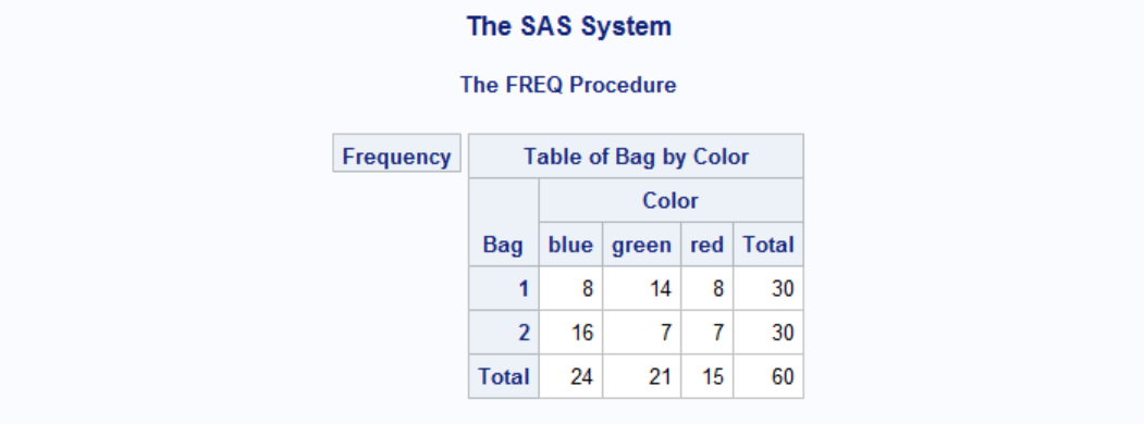
TABLE is major statement in PROC FREQ, it is somewhat similar to VAR statement in PROC MEANS. By requesting a table of Color, PROC FREQ calculates the frequecies of each color in the whole data set. If we instead want to see the frequency of colors in each bag we simply add Bag to our TABLE statement followed by a star * before Color argument.


If you find the output too crowded and eliminate some of the information, you can type these options in the TABLE statement. First, let's find out what information we do have. Take a look at the leftmost column in the ouput: Frequency, Percent, Row Pct, Col Pct. You can eliminate any of these with the following:


What if our data does not include individual marbles but exist as a contingency table like below?
| Bag | Color | Quantity |
|---|---|---|
| 1 | blue | 8 |
| 1 | green | 14 |
| 1 | red | 8 |
| 2 | blue | 16 |
| 2 | green | 7 |
| 2 | red | 7 |
In this case, we have to specify the quantity, i.e. WEIGHT:


Leave a Comment