Simple Linear Regression
Linear regression is a linear approach to modelling the relationship between a scalar response (or dependent variable) and one or more explanatory variables (or independent variables). The case of one explanatory variable is called simple linear regression.
Example: Self-Reports of Height and Weight
Description: Subjects were asked about their heights and weights and results are documented with measured heights and weights.
sex: A factor with levels: F, female; M, male.
weight: Measured weight in kg.
height: Measured height in cm.
repwt: Reported weight in kg.
repht: Reported height in cm.
errwt: Percent error of reported vs measured weight = (repwt-weight)/weight
errht: Percent error of reported vs measured height = (repht-height)/height
Source: https://vincentarelbundock.github.io/Rdatasets/doc/carData/Davis.html
Download the data from here
Task: Which gender estimates better?
Before digging into statistical analysis, let's first analyze the data with simple graphs.

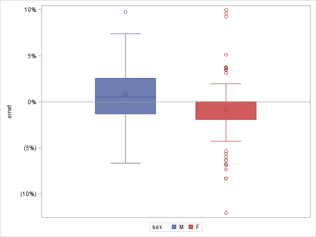
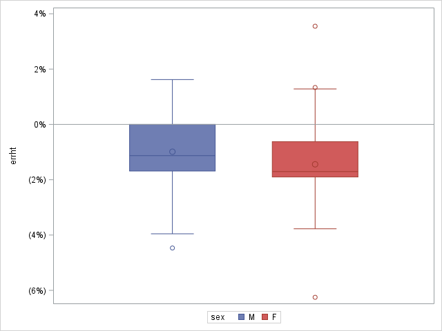
Above graph shows that females tend to underreport their weights and males tend to overreport. Both genders seem to underreport their heights.
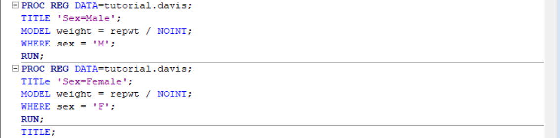
To determine which gender is more accurate in reporting their weight, we can run two separate regressions with each gender and then determine which one is more accurate based on regression output. SAS lets us run any procedure with a subset of dataset with a WHERE statement, quite similar to SQL.
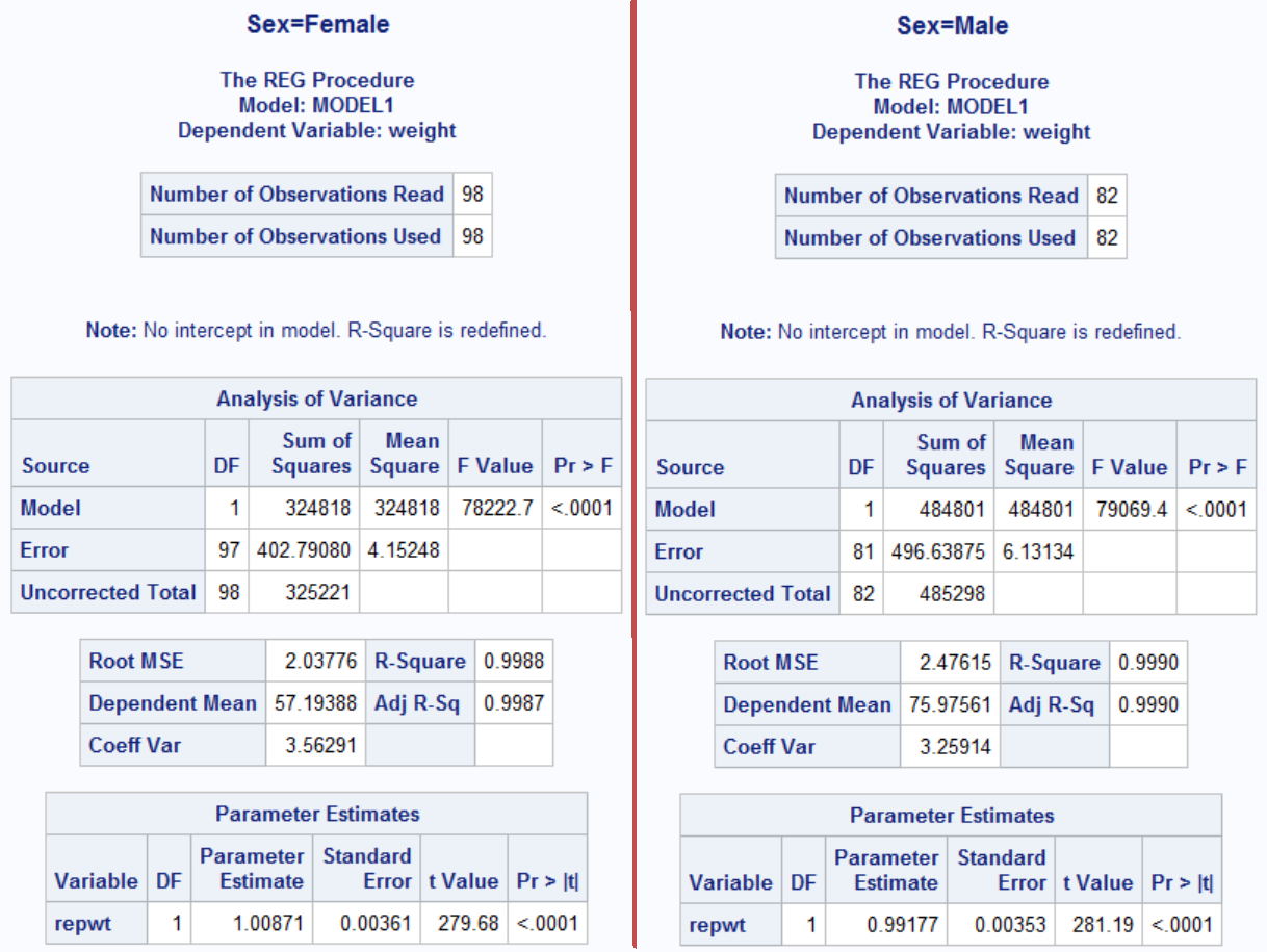
Parameter estimates show that females slightly underestimate (1.00871) whereas males slightly overestimate (0.99177), confirming our graphical analysis before. Now, let's go through our worth talking about regression outputs one by one.
Analysis of Variance: All output in this section tests the hypothesis that none of the independent variables have an effect on the dependent variable.
- - Source: The source of variation of the data. Is it from the model (Model), random variations (Error), or total (Corrected Total)
- - Pr > F: Also known as p-value. This gives us the probability that the coefficients are all equal to zero. Smaller the number, better our model.
Root MSE: The root mean squared error, which is the square root of the average squared distance of a data point from the fitted line. This value is higher for the model with the males mostly because male weights are larger so the errors tend to be larger.
Coeff Var: The coefficient of variation, which is the ratio of the Root MSE to the mean of the dependent variable. Since it is unitless, it can be used to compare two different models as opposed to Root MSE. This value is lower for the model with males, indicating better regression fit. In other words males' reported weights are closer to the measured values compared to females.
R-Square: This number is the most popular measure of how good our regression model in terms of explaining the variation in the data. R-Square is always between 0 and 1. R-Square values are 0.99 for our models which means 99% of the variation in the data can be explained by our model. In practice, this is as good as it gets and you rarely get such high values.
Adj R-Sq: Adjusted R-Square is the value of R-Square after adjusting for the nnumber of independent variables. Adding a new independent variable ALWAYS increases R-Square, never decreases. But if you add an irrelevant independent variable, Adj. R-Square decreases. That way we can figure out whether adding that independent variable is a good choice or not.
Parameter Estimates: This section is all about how good each of our independent variables are.
Pr > F: This number shows whether our independent variable is worth keeping in the model. Typically we want this number to be less than 0.05. In our case we have only one independent variable so it's irrelevant here.
Example: House Prices
Description: This dataset contains selling prices for 20 houses that were sold in 2008 in a small midwestern town. The file also contains data on the size of each house (in square feet) and the size of the lot (in square feet) that the house is on.
price: Selling price in dollars
size: Size of the house in square feet.
lot: Area of the houses lot in square feet.
Source: https://vincentarelbundock.github.io/Rdatasets/doc/Stat2Data/Houses.html
Download the data from here
Task: Develop a model to estimate price given size and lot.
Let's begin our first estimate by including all the variables (size and lot).
								PROC REG DATA = tutorial.houses;

								MODEL price = size lot;

								RUN;
| Number of Observations Read | 20 |
|---|---|
| Number of Observations Used | 20 |
| Analysis of Variance | |||||
|---|---|---|---|---|---|
| Source | DF | Sum of Squares |
Mean Square |
F Value | Pr > F |
| Model | 2 | 48048189470 | 24024094735 | 10.69 | 0.0010 |
| Error | 17 | 38196058530 | 2246826972 | ||
| Corrected Total | 19 | 86244248000 | |||
| Root MSE | 47401 | R-Square | 0.5571 |
|---|---|---|---|
| Dependent Mean | 159140 | Adj R-Sq | 0.5050 |
| Coeff Var | 29.78554 |
| Parameter Estimates | |||||
|---|---|---|---|---|---|
| Variable | DF | Parameter Estimate |
Standard Error |
t Value | Pr > |t| |
| Intercept | 1 | 34122 | 29716 | 1.15 | 0.2668 |
| Size | 1 | 23.23240 | 17.70041 | 1.31 | 0.2068 |
| Lot | 1 | 5.65654 | 3.07533 | 1.84 | 0.0834 |
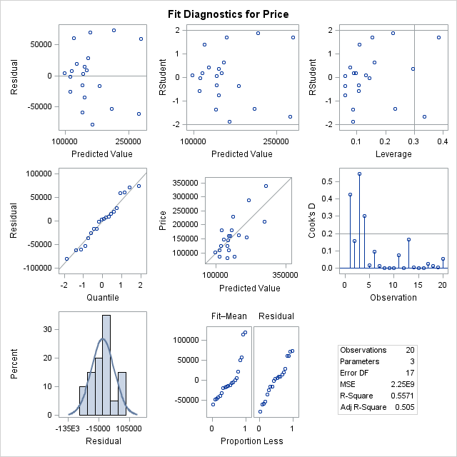
p-value for F-test is 0.0100 therefore model is statistically significant whereas p-values for our parameters all are above 0.05. Our R-Sq value is 0.5571 which means our model can explain 56% of the variation in house prices. Our model formula is price = 34,122 + 23.23*Size + 5.66*Lot.
Distribution of residuals vs predicted value is random which shows that our linearity estimation is correct. Extreme observations identified by Student's residual are below |2| - outlier is no concern.

Lrrr
Senior blog writer
Lrrr, ruler of the planet Omicron Persei 8, is a middle-aged Omicronian man with a bad temper and soft spots for the conquering of planets and 20th century television.
Popular Posts

Space The Final Frontier
02 Hours ago

The Amazing Hubble
02 Hours ago

Astronomy Or Astrology
02 Hours ago

Asteroids telescope
02 Hours ago

Leave a Comment