
Survival Analysis
Survival analysis is a branch of statistics for analyzing the expected duration of time until one or more events happen, such as death in biological organisms and failure in mechanical systems. This topic is called reliability theory or reliability analysis in engineering, duration analysis or duration modelling in economics, and event history analysis in sociology. Survival analysis attempts to answer questions such as: what is the proportion of a population which will survive past a certain time? Of those that survive, at what rate will they die or fail? Can multiple causes of death or failure be taken into account? How do particular circumstances or characteristics increase or decrease the probability of survival?
Survival analysis involves the modelling of time to event data; in this context, death or failure is considered an "event" in the survival analysis literature – traditionally only a single event occurs for each subject, after which the organism or mechanism is dead or broken.
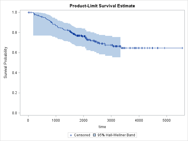
Let's look at the malignant melonoma survival data from here. Data set contains time, survival time in days, status (1: died from melanoma, 2: alive, 3: dead from other causes), sex (1: male 0: female) and ulcer (1: present, 0: absent). Download the data from here.
Here is the basic code to run a survival analysis:

TIME statement specifies the time variable and STATUS specifies whether the event is censored or not. We know that only status=1 denotes death from melanoma, 2 and 3 are censored data. Here is the survival plot from the output:


In order to see confidence bands, we need to specify what type of confidence band we'd like to see. Choices are Hall-Wellner (HW) and Equal Precision (EP)

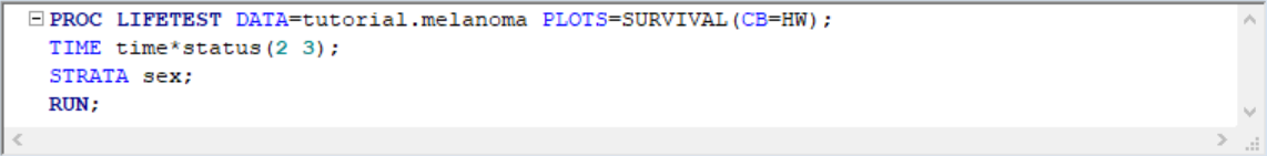
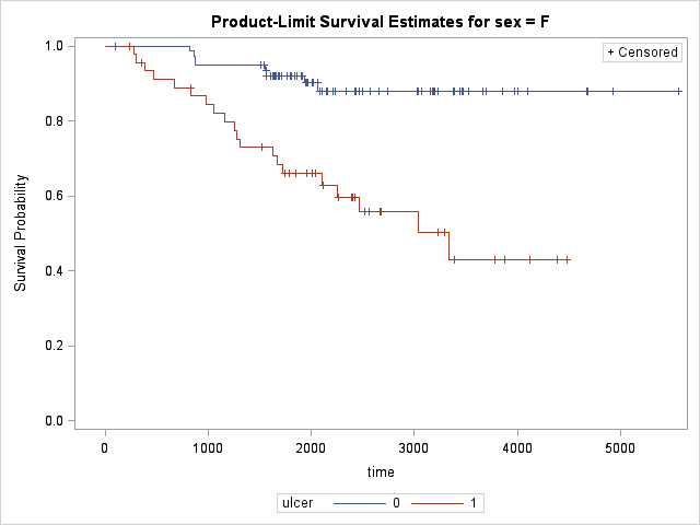
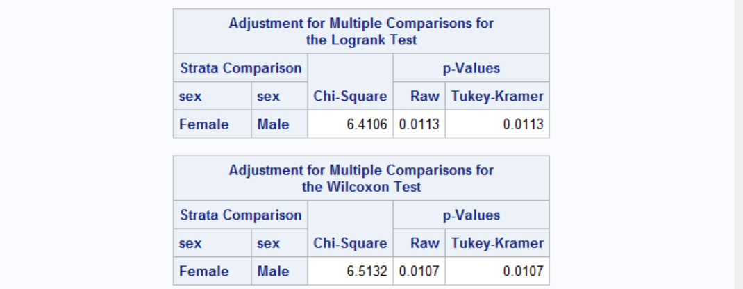
To see the effects of sex on survival, we can specify it as a STRATA:
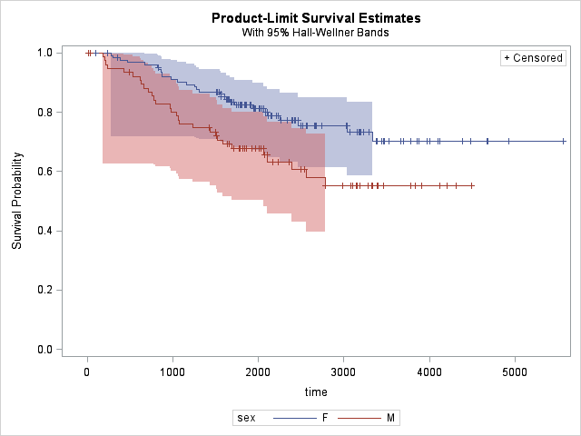
As can be seen from the survival plot, females have longer survival times compared to males. But let's also get some test values to comment. We can add TUKEY test to our comparison of males and females. Here's how it's done with the results:

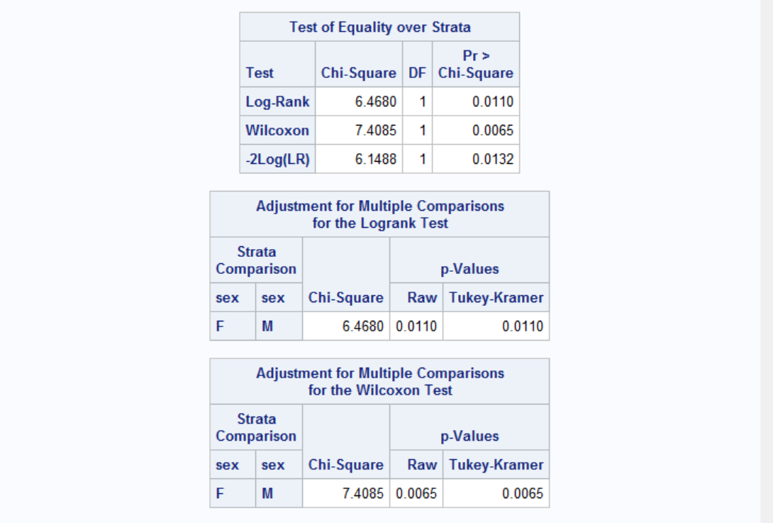
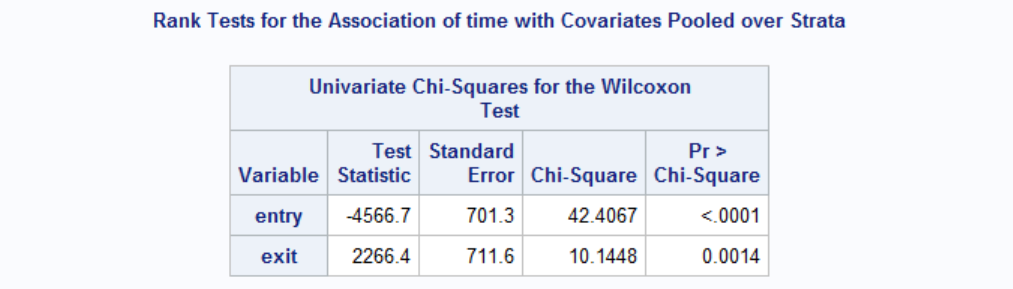
Results are shown for both Logrank and Wilcoxon tests. Both tests have p-values less than 0.05 therefore the effect of gender is significant. Note that Wilocoxon test gives more weight on shorter survival times and the difference of survival between genders at early onset gives raise to more significant p-value to Wilcoxon compared to Log-Rank. Now let's see the effect of ulcer on survival times while adjusting for gender difference.

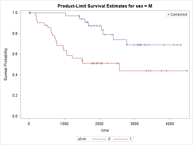
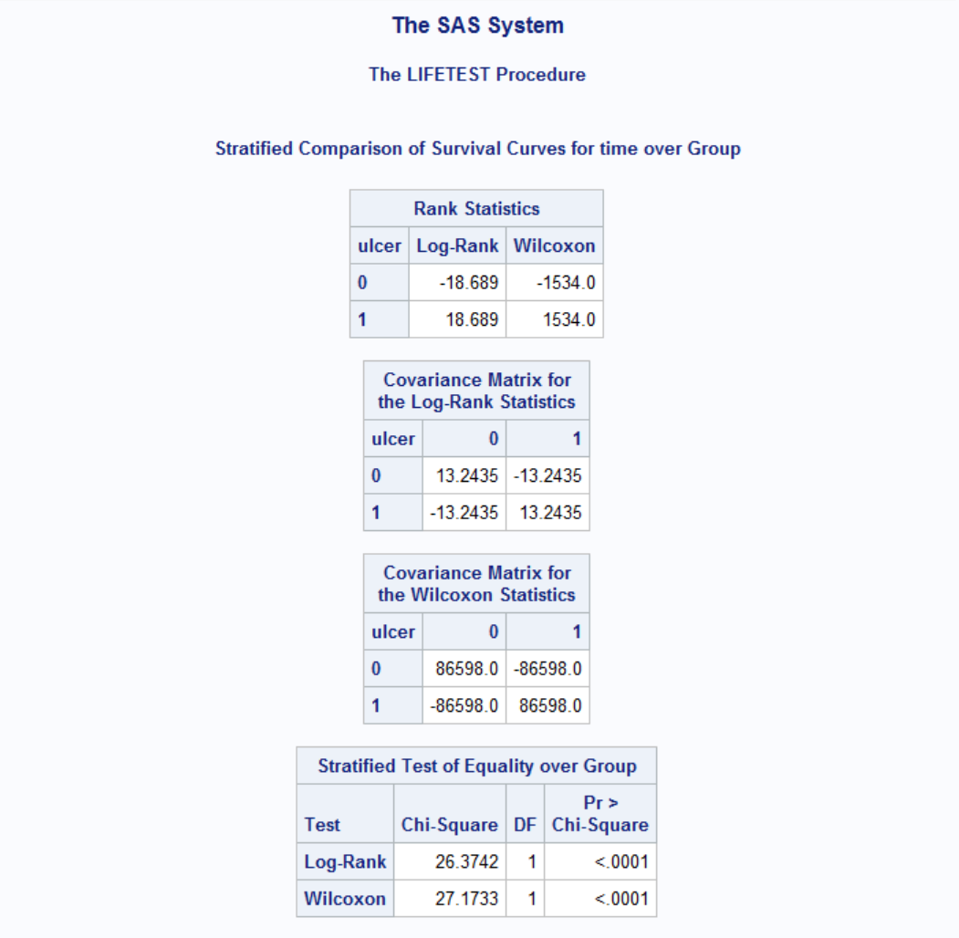
Results are highly significant and the effect of ulcer on different gender is evident as compared to gender-only test.
Example: Remission Times for Acute Myelogenous Leukaemia
Description: A clinical trial to evaluate the efficacy of maintenance chemotherapy for acute myelogenous leukaemia was conducted by Embury et al. (1977) at Stanford University. After reaching a stage of remission through treatment by chemotherapy, patients were randomized into two groups. The first group received maintenance chemotherapy and the second group did not. The aim of the study was to see if maintenance chemotherapy increased the length of the remission. The data here formed a preliminary analysis which was conducted in October 1974.
| time | cens | group |
| 9 | 1 | 1 |
| 13 | 1 | 1 |
| 13 | 0 | 1 |
| 18 | 1 | 1 |
| 23 | 1 | 1 |
| 28 | 0 | 1 |
| 31 | 1 | 1 |
| 34 | 1 | 1 |
| 45 | 0 | 1 |
| 48 | 1 | 1 |
| 161 | 0 | 1 |
| 5 | 1 | 2 |
| 5 | 1 | 2 |
| 8 | 1 | 2 |
| 8 | 1 | 2 |
| 12 | 1 | 2 |
| 16 | 0 | 2 |
| 23 | 1 | 2 |
| 27 | 1 | 2 |
| 30 | 1 | 2 |
| 33 | 1 | 2 |
| 43 | 1 | 2 |
| 45 | 1 | 2 |
time: The length of the complete remission (in weeks).
cens: An indicator of right censoring. 1 indicates that the patient had a relapse and so time is the length of the remission. 0 indicates that the patient had left the study or was still in remission in October 1974, that is the length of remission is right-censored.
group: The group into which the patient was randomized. Group 1 received maintenance chemotherapy, group 2 did not.
Source: https://vincentarelbundock.github.io/Rdatasets/doc/boot/aml.html
Download the data from here
Task: Analyze the dataset wrt survival times of group 1 and 2.

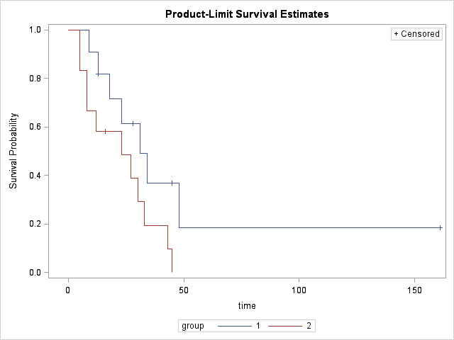
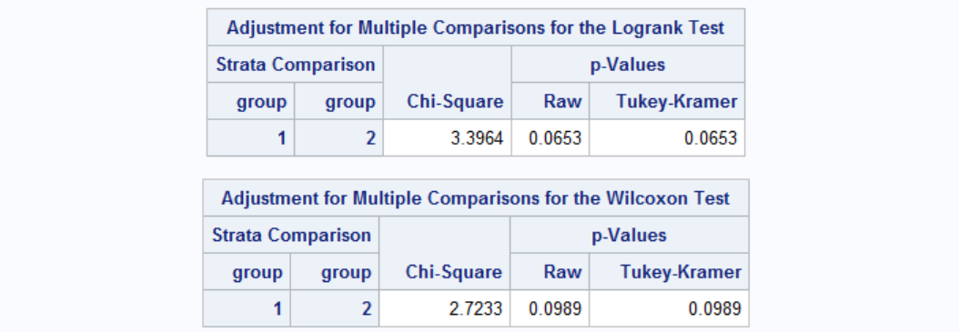
While the survival graph shows some difference between group 1 and 2, neither of the Wilcoxon or Log-Rank tests is significant. Therefore, the difference between the survial times of group 1 and 2 is not statistically significant at the 0.05 level.
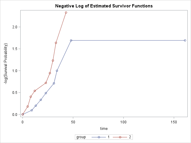
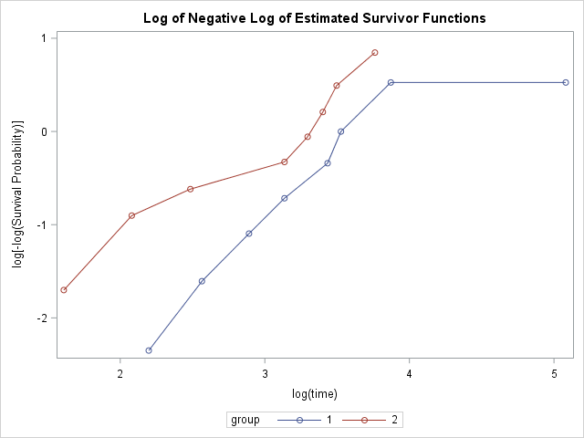
Let's also get Log and Log-Log survival plots in addition to Linear survival plot. We can do this by specifying the plots we would like to see in the PROC LIFETEST statement.
Example: Channing House Data
Description: Channing House is a retirement centre in Palo Alto, California. These data were collected between the opening of the house in 1964 until July 1, 1975. In that time 97 men and 365 women passed through the centre. For each of these, their age on entry and also on leaving or death was recorded. A large number of the observations were censored mainly due to the resident being alive on July 1, 1975 when the data was collected. Over the time of the study 130 women and 46 men died at Channing House. Differences between the survival of the sexes, taking age into account, was one of the primary concerns of this study.
sex: A factor for the sex of each resident ("Male" or "Female").
entry: The residents age (in months) on entry to the centre.
exit: The age (in months) of the resident on death, leaving the centre or July 1, 1975 whichever event occurred first.
time: The length of time (in months) that the resident spent at Channing House. (time=exit-entry).
cens: The indicator of right censoring. 1 indicates that the resident died at Channing House, 0 indicates that they left the house prior to July 1, 1975 or that they were still alive and living in the centre at that date.
Source: https://vincentarelbundock.github.io/Rdatasets/doc/boot/channing.html
Download the data from here
Task: Survival analysis along with testing covariates gender and age.
Let's first run our LIFETEST procedure in its simple form and see what our survival graph looks like.

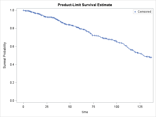
It looks like our linear survival assumption seems to be valid. Now we can test the effect of gender on survival.


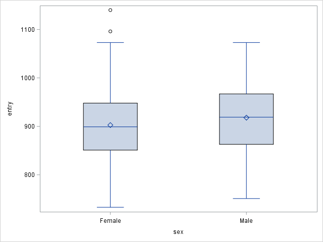
Effect of gender on survival is statistically significant. But what about the age? It may be possible that females survive longer because they are younger when they enter the house.
Effect of age is clearly significant for both genders. Therefore age effect is not favoring one gender over another. We can see this by testing age differences between females and males when they first enter the house. To do this, we can run a t-test with PROC TTEST.

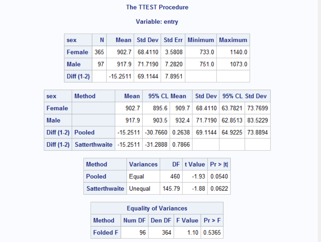
Results show that there is no significant age differences between males and females. The effect of gender on survival times is independent of the age, i.e. females survive longer than males.
Example: Customer Purchase
Description: Garden dataset contains 30,000 customers who were observed over a four year period. Their start time is when they make their first purchase. They are monitored until the end of the four year period.
id_number: Customer ID.
start: Customer's first purchase.
end: Customer's second purchase.
censor: 1 if there is a second purchase, 0 if not.
last_day: End of the study.
time: Number of months between first purchase and second or last day of study, whicever is smaller.
garden: Dollars spent in garden department of first purchase.
decorating: Dollars spent in decorating department of first purchase.
car: Dollars spent in auto department of first purchase.
electrical: Dollars spent in electrical department of first purchase.
safety: Dollars spent in safety department of first purchase.
computer: Dollars spent in computer department of first purchase.
previous_garden: Previous amount spent in garden tools.
previous_decorating: Previous amount spent in decorating tools.
previous_car: Previous amount spent in auto tools.
previous_electrical: Previous amount spent in electrical tools.
previous_safety: Previous amount spent in safety tools.
previous_computer: Previous amount spent in computer tools.
amount_clv: Total amount spent in customer lifetime.
strata: Strata based on total number of orders. A: 1-2 orders between 2011 and 2013, B: 1-2 orders in 2014, C: 3-4 orders, D: 5-10 orders, E: 11-20 orders, F: >21 orders.
account_origin: Channel where the account is originated.
order: Channel where the first purchase is made.
age: Binned age.
credit_score: Binned credit score.
behavior: Binned behavior.
mosaic: Mosaic bureau data.
credicard: Method of payment or credit card brand.
family: Family bureau data.
income: Income bureau data.
Source: Business Survival Analysis Using SAS, J. Ribeiro.
Download the data from here
Task: Design a model to predict the importance of covariates in survival.
The analysis of survival data requires special techniques because the data are almost always incomplete, and familiar parametric assumptions might be unjustifiable. Investigators follow subjects until they reach a prespecified endpoint (for example, death). However, subjects sometimes withdraw from a study, or the study is completed before the endpoint is reached. In these cases, the survival times (also known as failure times) are censored; subjects survived to a certain time beyond which their status is unknown. The uncensored survival times are sometimes referred to as event times. Methods of survival analysis must account for both censored and uncensored data.
Many types of models have been used for survival data. Two of the more popular types of models are the accelerated failure time model and the Cox proportional hazards model. Each has its own assumptions about the underlying distribution of the survival times. Two closely related functions often used to describe the distribution of survival times are the survivor function and the hazard function (see the section Failure Time Distribution for definitions). The accelerated failure time model assumes a parametric form for the effects of the explanatory variables and usually assumes a parametric form for the underlying survivor function. Cox’s proportional hazards model also assumes a parametric form for the effects of the explanatory variables, but it allows an unspecified form for the underlying survivor function.
The PHREG procedure performs regression analysis of survival data based on the Cox proportional hazards model. Cox’s semiparametric model is widely used in the analysis of survival data to explain the effect of explanatory variables on hazard rates.
Here's the code to find which covariates are important for survival, i.e. time.
								PROC PHREG DATA=tutorial.garden_sample;

								MODEL time*censor(0) = account_origin age amount_clv strata income computer credicard credit_Score decorating electrical family garden mosaic order prev_car prev_computer prev_decorating prev_electrical prev_garden prev_safety safety / SELECTION=STEPWISE;

								RUN;
| Summary of Stepwise Selection | |||||||
|---|---|---|---|---|---|---|---|
| Step | Effect | DF | Number In |
Score Chi-Square |
Wald Chi-Square |
Pr > ChiSq | |
| Entered | Removed | ||||||
| 1 | Strata | 5 | 1 | 12052.1093 | <.0001 | ||
| 2 | Credit_score | 4 | 2 | 273.1409 | <.0001 | ||
| 3 | Prev_Garden | 1 | 3 | 84.6997 | <.0001 | ||
| 4 | Order | 2 | 4 | 48.3254 | <.0001 | ||
| 5 | Account_Origin | 3 | 5 | 74.4897 | <.0001 | ||
| 6 | Safety | 1 | 6 | 21.5602 | <.0001 | ||
| 7 | Prev_Decorating | 1 | 7 | 31.6292 | <.0001 | ||
| 8 | Decorating | 1 | 8 | 11.6206 | 0.0007 | ||
| 9 | Prev_Car | 1 | 9 | 9.0293 | 0.0027 | ||
| 10 | Credicard | 5 | 10 | 12.3538 | 0.0302 | ||
| 11 | Income | 1 | 11 | 4.4819 | 0.0343 | ||
| 12 | Computer | 1 | 12 | 4.0999 | 0.0429 | ||
Example: Chemotherapy for Stage B/C colon cancer
Description: These are data from one of the first successful trials of adjuvant chemotherapy for colon cancer. Levamisole is a low-toxicity compound previously used to treat worm infestations in animals; 5-FU is a moderately toxic (as these things go) chemotherapy agent. There are two records per person, one for recurrence and one for death.
id: Patient ID.
study: 1 for all patients.
rx: Treatment - Obs(ervation), Lev(amisole), Lev(amisole)+5-FU.
sex: 1=male, 0=female.
age: Age in years.
obstruct: Obstruction of colon by tumour.
perfor: Perforation of colon.
adhere: Adherence to nearby organs.
nodes: Number of lymph nodes with detectable cancer.
time: Days until event or censoring.
status: Censoring status.
differ: Differentiation of tumour (1=well, 2=moderate, 3=poor).
extent: Extent of local spread (1=submucosa, 2=muscle, 3=serosa, 4=contiguous structures).
surg: Time from surgery to registration (0=short, 1=long).
node4: More than 4 positive lymph nodes.
etype: Event type: 1=recurrence,2=death.
Source: https://vincentarelbundock.github.io/Rdatasets/doc/survival/colon.html
Download the data from here
Task: Design a model to predict the importance of covariates in survival.
Let's first take a look at recurrence with different treatments:
								PROC LIFETEST DATA=tutorial.colon PLOTS=HAZARD;

							TIME time*status(0);

							STRATA rx;

								WHERE etype=1;

								RUN;
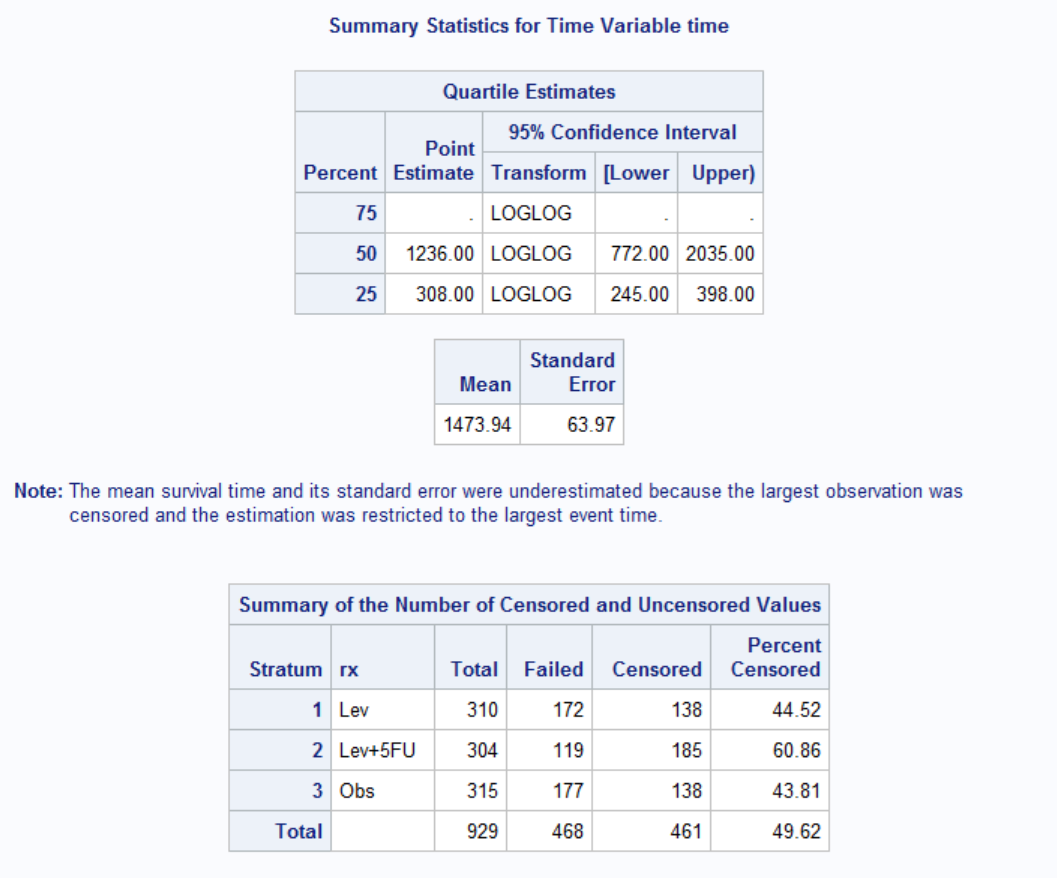
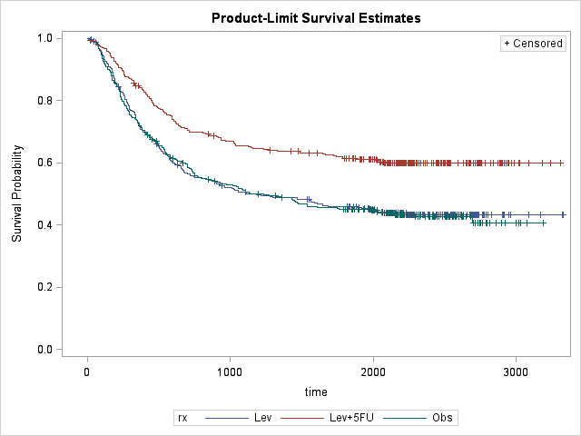
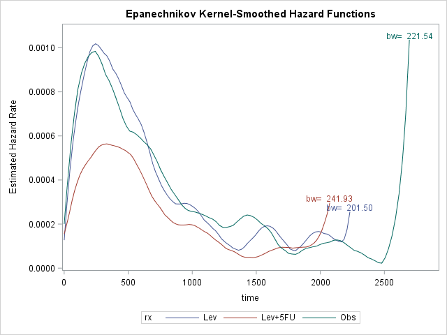
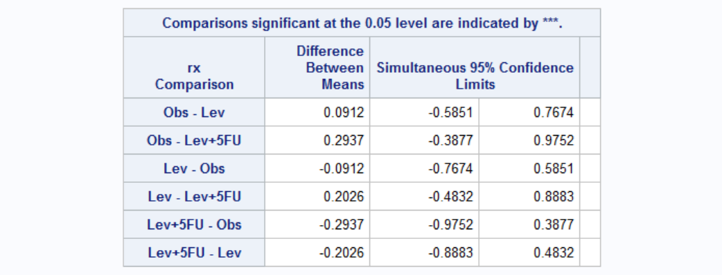
Mean survival time is 1474 days, i.e. average time before recurrence occurs is about 4 years. Survival plot shows that rx=Lev+5FU seems effective whereas Lev alone is not effective. Also hazard plot shows that majority of the recurrence occur around 400 days, ~1 year, regardless of the treatment received. After that there is a slightly increased risk around 1400 days, particularly for rx=Obs and rx=Lev. It seems like recurrence would not likely occur if it does not occur within first 4 years.
Now let's analyze the survival till death.
								PROC LIFETEST DATA=tutorial.colon PLOTS=HAZARD;

								TIME time*status(0);

								STRATA rx;

								WHERE etype=2;

								RUN;
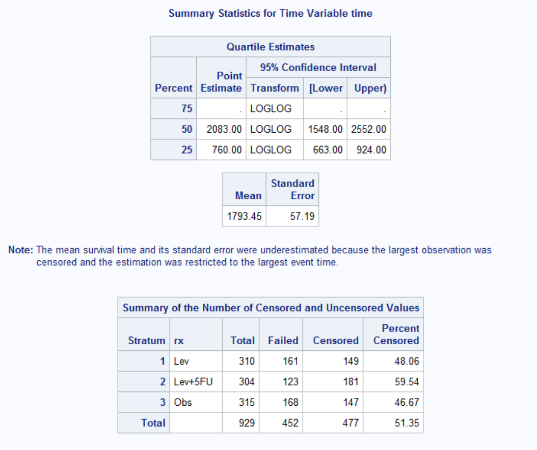
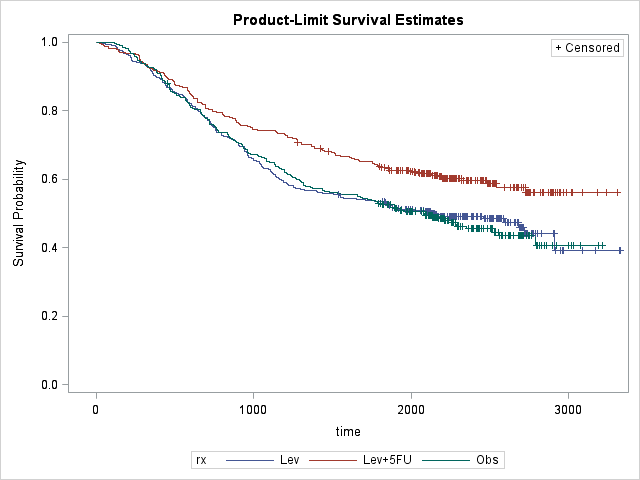
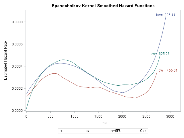
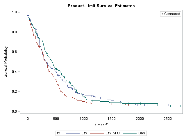
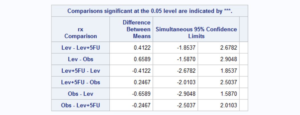
Average survival time with Stage B/C colon cancer is around 1793 days, i.e. about 5 years. Again rx=Lev+5FU seems to be effective in survival. The biggest risk for death is around 600 for Lev+5FU and around 800 otherwise. This might be because the patients who are treated with Lev+5FU are already in more serious condition than others. Regardless, hazard rate for patients with Lev+5FU is clearly lower, i.e. these patients are more likely to survive.
Let's now see the effect of gender/rx combination.
								PROC LIFETEST DATA=tutorial.colon PLOTS=HAZARD;

								TIME time*status(0);

								STRATA rx;

								WHERE etype=2;

								RUN;
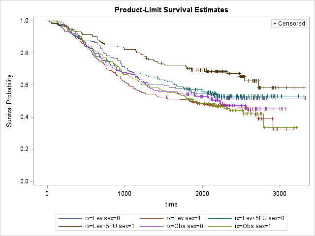
Interestingly, it seems like Lev+5FU is more effective on male patients. However to understand the effect of covariates we need to use another tool, PHREG:
PROC PHREG DATA=tutorial.colon;
CLASS rx(REF='Obs') differ(REF='1') extent(REF='1') surg(REF='0') sex obstruct perfor adhere;
MODEL time*status(0) = rx|sex obstruct perfor adhere differ extent surg nodes / SELECTION=STEPWISE SLENTRY=0.25 SLSTAY=0.05;
HAZARDRATIO 'H1' nodes / UNITS=1 CL=BOTH;
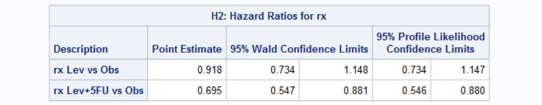
HAZARDRATIO 'H2' rx / DIFF=REF CL=BOTH;
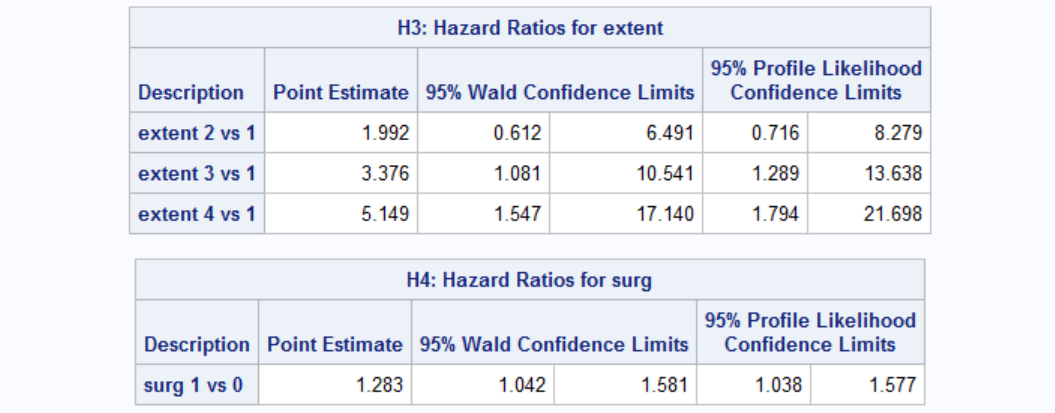
HAZARDRATIO 'H3' extent / DIFF=REF CL=BOTH;
HAZARDRATIO 'H4' surg / DIFF=REF CL=BOTH;
WHERE etype=2;
RUN;
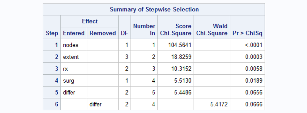
Results of stepwise selection of covariables are below. Covariables nodes, extent, rx, surg are significant whereas others are not (Note I ran this analysis before that's why I specified HAZARDRATIO for the selected variables only - it would not be apparent at first to you.).
Let's look at the hazard ratio for nodes below. Hazard ratio results tell us that every additional malignant nodes increases the chance of death by 1.094 times in a given time period. A patient with 4 nodes is 1.094x1.094x1.094 = 1.31 times more likely to die than a patient with only 1 node.

Hazard ratios for treatment below shows that Lev alone is not effective (by 95% confidence) because confidence level includes 1. Lev+5FU, on the other hand, is clearly effective.
You can see below the hazard ratios for extent and surg. Interpretation of the results are similar.
While the analysis seemed to reach a conclusion we are still missing a certain piece: what are the chances of survival after the disease is recurred? Our dataset includes time to death which is the time beginning from the first time disease is discovered. Time to death after recurrence is thus td-tr, where td and tr are the time to death and time to recurrence, respectively. Our dataset does not offer this info readily so we have to utilize PROC SQL to reformat our dataset so that we can use it for further analysis.
								PROC SQL;

								CREATE TABLE colon_new AS

								SELECT a.id,

       a.rx,

       a.sex,

       a.age,

       a.obstruct,

       a.perfor,

       a.adhere,

       a.nodes,

       a.status AS statusd,

       b.status AS statusr,

       a.differ,

       a.extent,

       a.surg,

       a.node4,

       a.time AS timetodeath,

       b.time AS timetorec,

       a.time-b.time AS timediff

							FROM tutorial.colon a JOIN tutorial.colon b ON a.id=b.id

							WHERE a.etype = 1 AND b.etype = 1

								;

								QUIT;
Now we can invoke LIFETEST to get a first glance at our survival:
								PROC LIFETEST DATA=colon_new PLOTS=HAZARD;

								TIME timediff*statusd(0);

								STRATA rx;

							RUN;
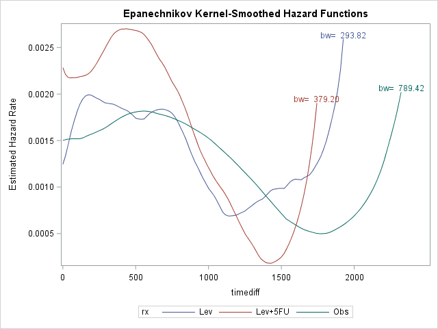
We can clearly see that once the recurrence is occured treatment has little effect, if any. It looks like once the disease recur, death is most likely within 700-800 days. Let's try to quantify our effects with PHREG:
								PROC PHREG DATA=tutorial.colon;

								CLASS rx(REF='Obs') differ(REF='1') extent(REF='1') surg(REF='0') sex obstruct perfor adhere;

								MODEL timediff*statusd(0) = rx|sex obstruct perfor adhere differ extent surg nodes / SELECTION=STEPWISE SLENTRY=0.25 SLSTAY=0.05;

								HAZARDRATIO 'H1' nodes / UNITS=1 CL=BOTH;

								HAZARDRATIO 'H2' rx / DIFF=REF CL=BOTH;

								HAZARDRATIO 'H3' sex / DIFF=REF CL=BOTH;

								HAZARDRATIO 'H4' age / UNITS=5 CL=BOTH;

								RUN;
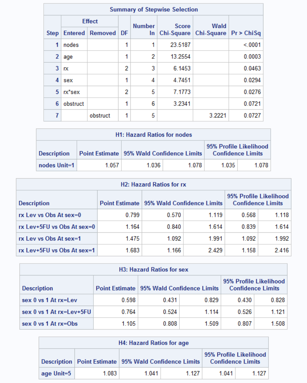
Again the number of nodes is the most important parameter in survival once the disease is recurred. Each additional node increases the odds of death 1.057 times. Effect of treatment seems to be dependent on the gender. Treatment has no effect on women (both Lev and Lev+5FU have confidence limits including 1, middle point). For men, treatment seems to be have a negative effect. However this might be because more serious patients actually receive treatment. Let's see for example whether patients older or with high number nodes received different treatments by ANOVA.
Looks like the effect is real: treatment has a negative effect once the disease is recurred. Age also has a negative effect on survival: every 5 additional year increases the odds of death by 1.083.

Lrrr
Senior blog writer
Lrrr, ruler of the planet Omicron Persei 8, is a middle-aged Omicronian man with a bad temper and soft spots for the conquering of planets and 20th century television.
Popular Posts

Space The Final Frontier
02 Hours ago

The Amazing Hubble
02 Hours ago

Astronomy Or Astrology
02 Hours ago

Asteroids telescope
02 Hours ago

Leave a Comment